Heat Transfer Problem
Heat transfer occurs only within a solid or fluid
Heat transfer occurs between multiple, separate, layers
Heat transfer occurs within a solid and into a liquid
Heat transfer only occurs between a solid and fluid
Conduction
Conduction is the transfer of heat through collisions between atoms/molecules and the diffusion of atoms/molecules of high energy. It is mainly defined by Fourier's Law.
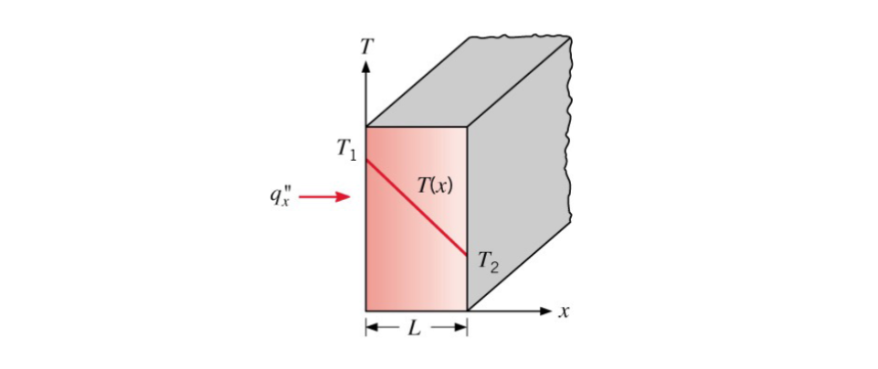
It can occur inside a fluid or a solid. See ME3304 S24 Lecture Note (1) Introduction for more info.
One Dimensional
For one-dimensional (x direction only), steady-state, heat diffusion we find that depends on the temperature difference across the solid, the area perpendicular to the flow -
Thus we can calculate the heat transfer rate as the following:
Again,
We call
We can convert this to heat flux by moving the area over.
Two Dimensional
With Heat Generation
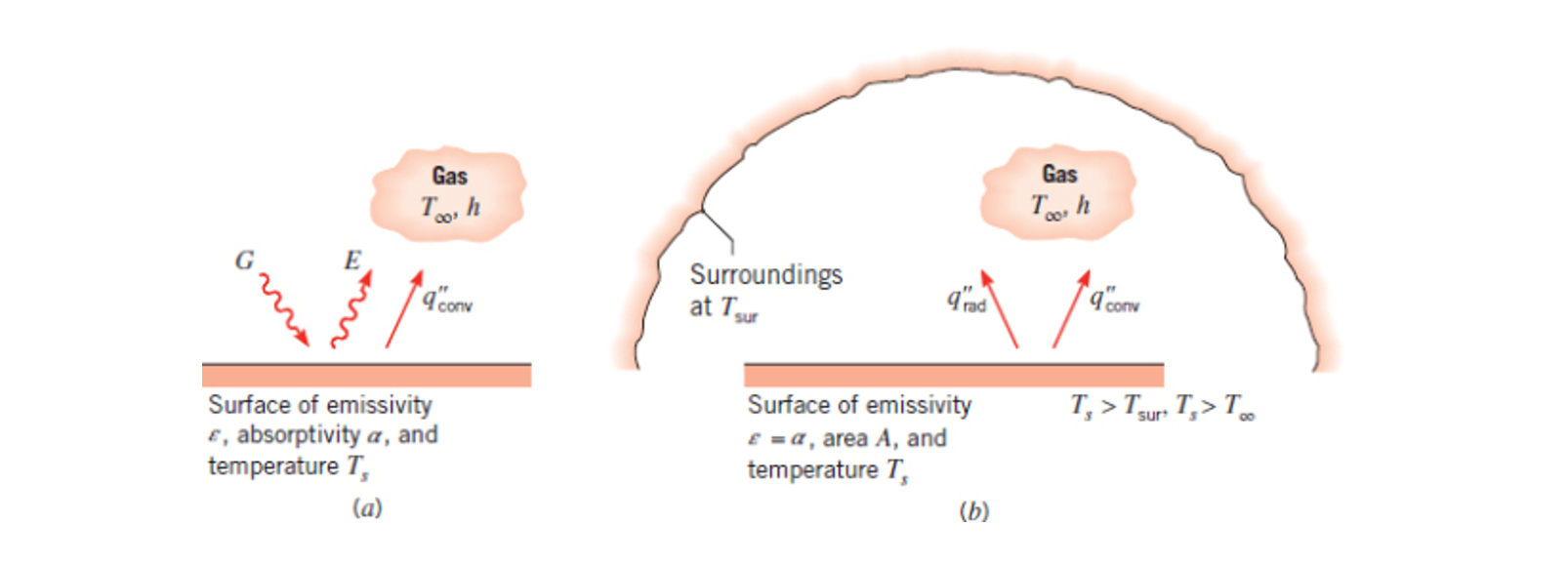
Convection
Convection is heat transfer from a solid to a liquid or vise-versa. It is driven by diffusion.
It is given by the following equation:
Where
Fluid Flow
Chapter 6 reviews convection in depth, fluid flow concepts are heavily involved in this chapter.
Finite Difference Analysis
Finite Difference Analysis, also known as finite-element or boundary-element, is a method of analysis that use finite values rather than the continuous ones of other methods.
It is an approximation rather than an exact result.
This method makes use of a nodal network to break a solid up into finite elements.
See the following for examples and more information:
Fourier's Law
Fourier's Law essentially states that heat flux is always normal to a cross sectional area of constant temperature.

Where
See ME3304 S24 Lecture Note (1) Introduction for more information.
Radiation
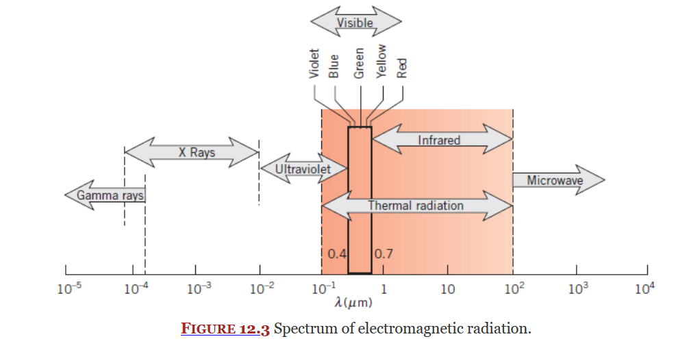
Covered in Chapter 12 and 13, radiation is heat transfer due to changes in election configuration, it takes the form of electromagnetic waves.
Radiation exists on electromagnetic radiation spectrum (Figure 12.3 below), a subset of this spectrum is thermal radiation which is what this course focuses on. Thermal radiation is an electromagnetic wave.
From 13E - 2nd Class:
Thermal radiation is measured via four different radiation heat fluxes defined in table 12.1:
See ME3304 S24 Lecture Note (7) Radiation for more info.
When working with radiation, Dr. Paul recommends to always convert to Kelvin.
Extended Surfaces (Fins)
Extended Surfaces or Fins are sections of an object that extend out into a fluid used for heat dissipation. They are covered in Section 3.6.
General form of energy dissipation equation for a fin (Eq. 3.66):
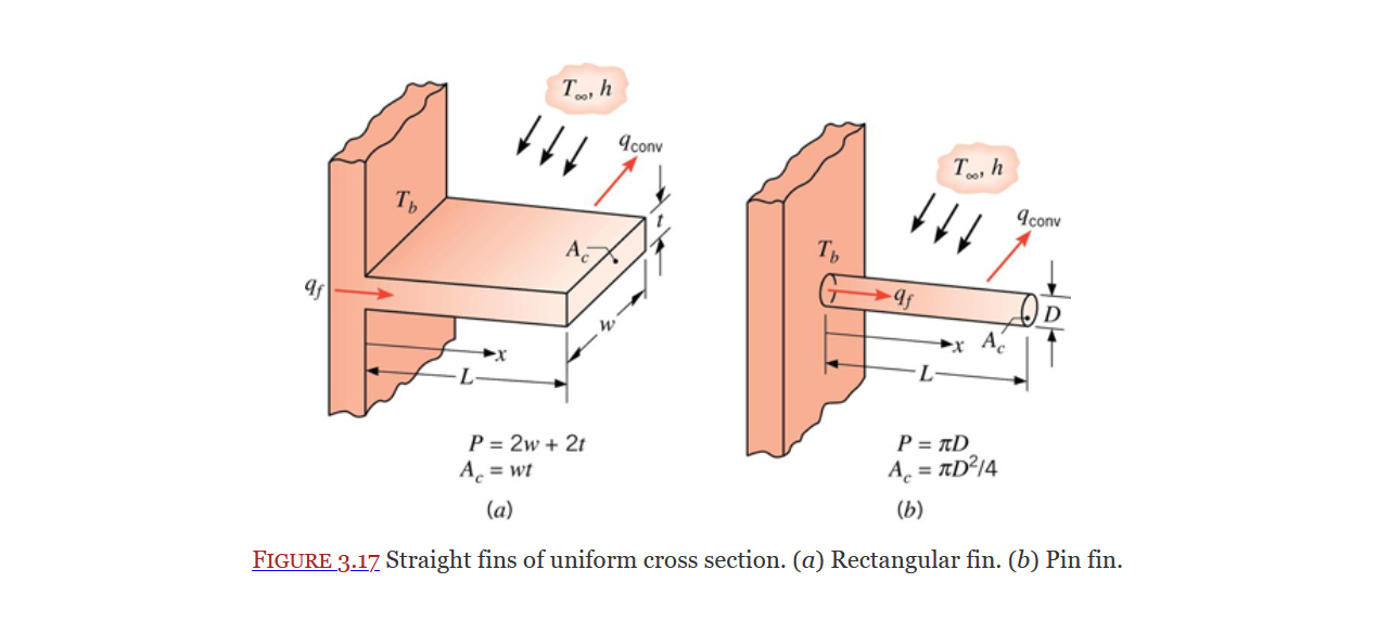
In the above image the cross section does not change along the length of the fin, thus the general equation can be reduced to the following (Eq. 3.67):
The following two definitions (Eq. 3.68 & 3.70):
allow us to reduce our equation (Eq. 3.69):
Now that it is in this form we can find it's general solution to be (Eq. 3.71):
We generally refer to
A derivation for a rod fin can be found in 4E - Class 2 - Fins Cont. 2024-02-13 00_10_36
Hyperbolic tribometry functions (namely
See extended-surface-equation-table for equations related to extended surfaces.
Energy Balance
Heat Transfer lives as a subcategory of thermodynamics and is based off its ideas. Energy balance is one of thermodynamics' defining characteristics and is true for heat transfer.
Starting with the a basic energy balance about a control volume we have:
Where
We can develop this further by accounting for energy stored within a control-volume and energy generated by a control volume using the following equation:
See Section 1.3 of the textbook for more information.
This concept is applied to systems using conduction by the heat diffusion equation.
Heat Diffusion Equation
Equation 2.19 (below) is the general form of the heat diffusion equation in cartesian coordinates.
Where
Cylindrical Coordinates (Eq. 2.26 - Pg. 65)::
Spherical Coordinates (Eq. 2.29 - Pg. 67):
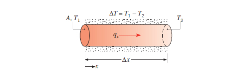
Thermal Circuits
In many cases heat flow can be analyzed using thermal 'circuits'. When using this approach heat transfer rate becomes current, temperature difference becomes voltage, and resistance is the material's resistance to the heat flow.
Thermal circuits are covered in chapter 3.
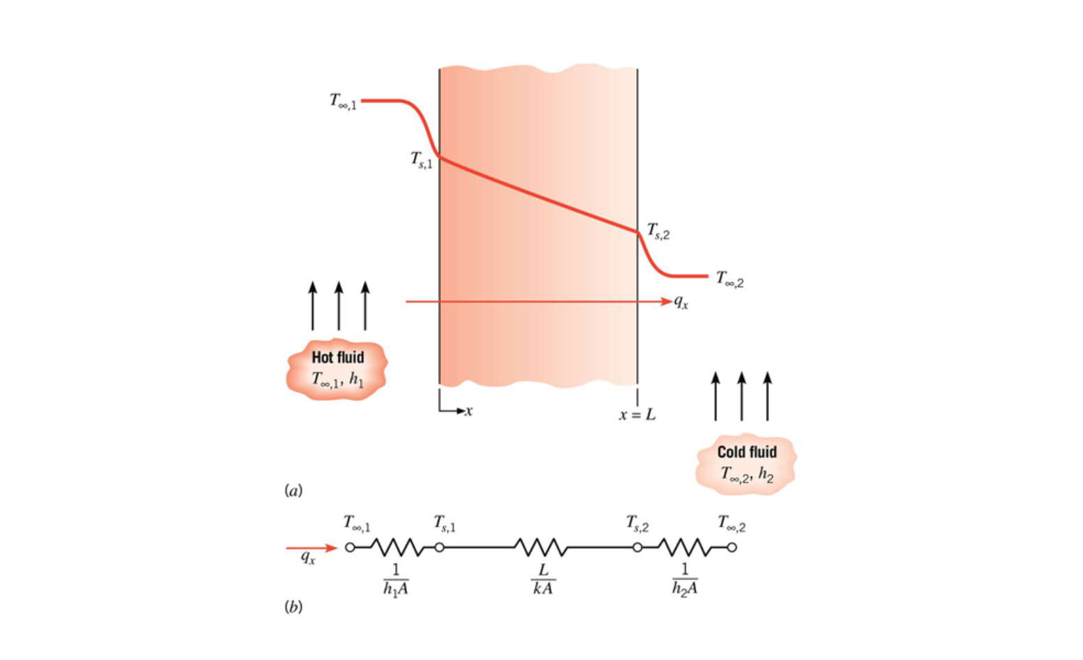
Resistance for conduction:
Where
Resistance for convection:
Where
Contact Resistance
Section 3.1.4
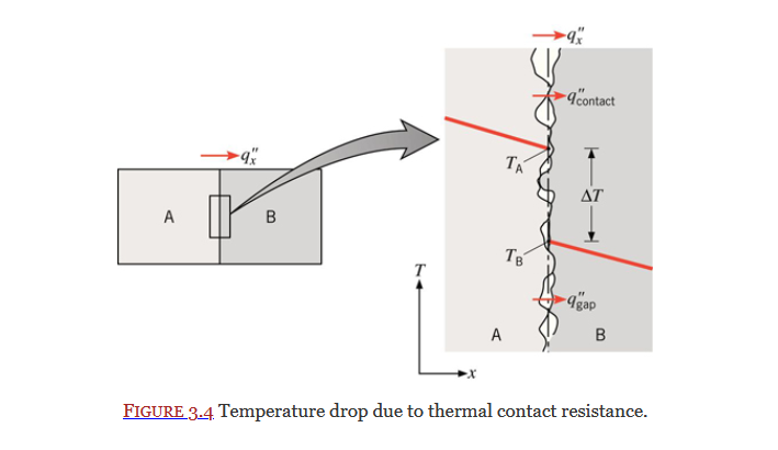
Equation 3.20:
Thermal Capacitance
Thermal capacitance is an idea that builds upon the foundations laid down in thermal circuits. It is explained in its own page.
Problem is a function of only time (not space/location)
Lumped Capacitance Method
Lumped Capacitance really means that heat transfer is a function of time only.
- Dr. Paul
Lumped Capacitance Method is a continuation of the ideas laid down in thermal circuits. As the name suggests we now have a thermal capacitance,
This method is an approximation and it only works is there is no temperature gradient across the object. This can be quantified by checking to make sure the biot number is much smaller than 1. See ME3304 S24 Lecture Note (2) Conduction.
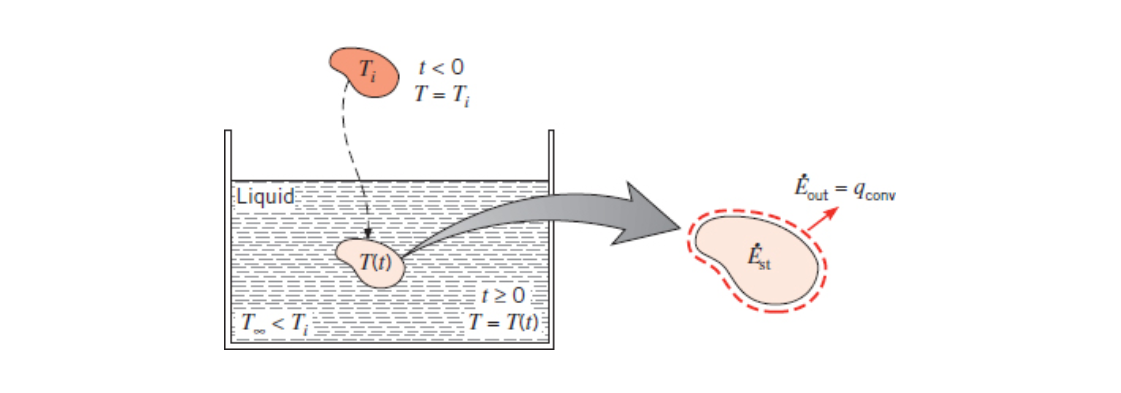
Given a solid of a high temperature that is in an environment that rapidly changes temperature (for example heat treating metal) we imagine that the solid is a capacitor (or battery). As soon as our solid changes environment it will start to discharge its energy as heat.
Equation 5.4 (temperature difference):
Equation 5.5:
Where
Equation 5.6:
See also ME3304 S24 Lecture Note (2) Conduction.
Where
Relating to thermocouple somehow.
An example of a problem using this method can be found in ME3304 Conduction Previous Test Solution.
Allows you to write energy-stored as the following?
Semi Infinite Solid
A method that considers space and time.
- Dr. Paul
In contrast to lumped capacitance method which only works on problems that are a function of time, semi-infinite solid method works on problems that are a function of both location and time.
Semi-Infinite Solid is an analysis method that uses a solid that is of infinite size in all but one direction. It is used to analyze temperature of an object over time.
This method yields an analytical solution rather than an approximation, although you are still making an approximation in the fact that infinite solids do not exist. Unlike the lumped capacitance method it can be used where there is a temperature gradient across the solid we are analyzing (the biot number is not very small).
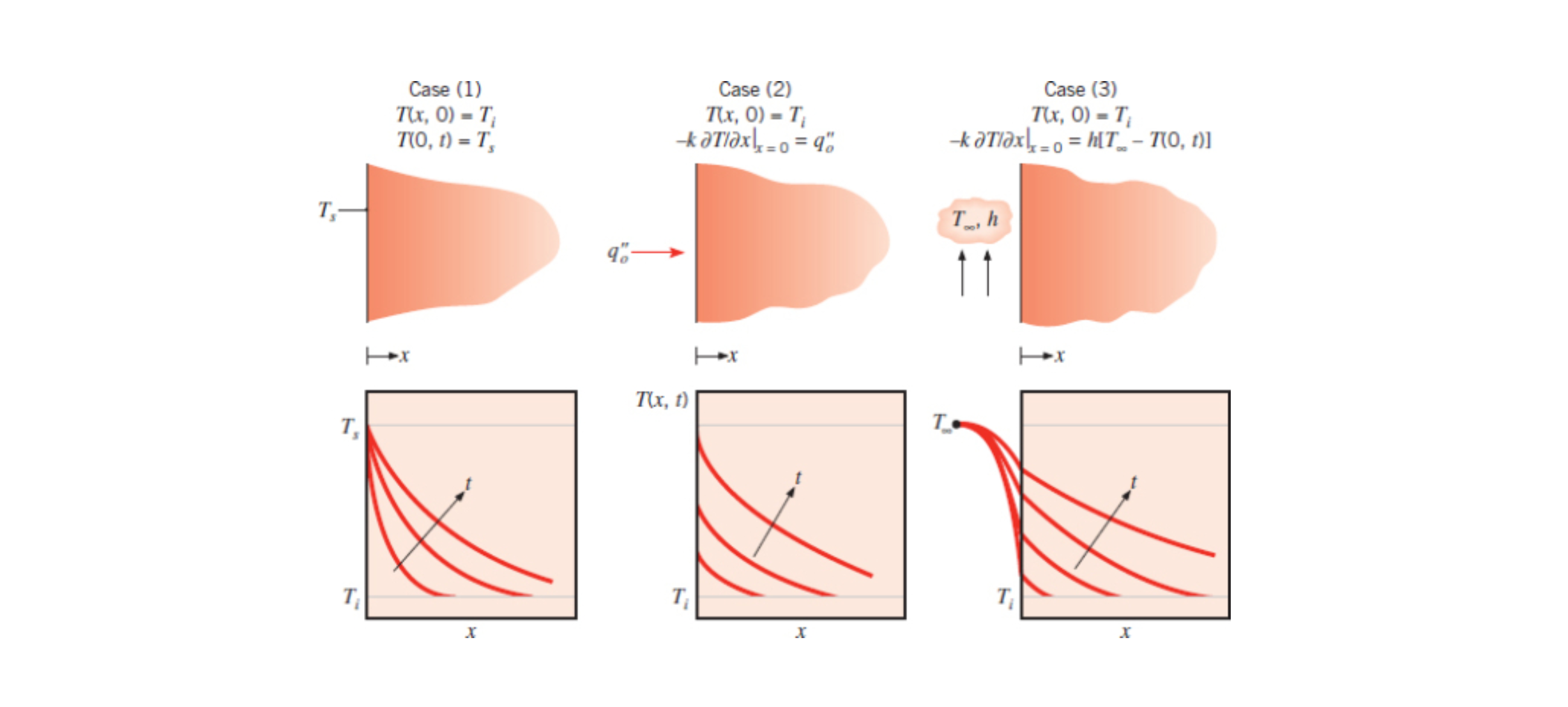
Below are example transient temperature distribution for constant surface temperature (1), constant surface heat flux (2), and surface convection (3).
See Section 5.7, 6E - Class 2, 7A - 2nd Class, and 7C - 2nd Class.
Temperature distribution
The derivation for the following equations (and what the error function is and where it came from) can be found in 7A - 2nd Class.
Equation 5.60:
Where
Case 1 Constant Surface Temperature (Eq. 5.61):
Case 2 Constant Surface Heat Flux (Eq. 5.62):
Case 3 Surface Convection (Eq. 5.63):
Where
Python
Equation 5.63 (Case 3 above):
def caseThree(T, Ti, Too, x, alpha, t, h, k):
coeffOne = erfc(x/(2*sqrt(alpha * t)))
coeffTwo = exp(((h*x)/k) + ((h**2 * alpha*t)/k**2))
coeffThr = erfc((x/2*sqrt(alpha*t)) + ((h*sqrt(alpha*t))/k))
coeffFou = (T-Ti)/(Too-Ti)
return coeffOne - coeffTwo * coeffThr - coeffFou
Problem is a function of both time and space (location)
Internal Flow
Chapter 8
Internal fluid flow is fluid flow that occurs within a pipe or other container.
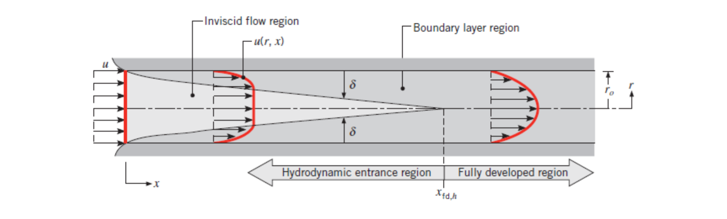
If the flow is laminar (ie. in the fully developed region) the velocity profile is parabolic. See entry-region for how to calculate the distance at which the fully developed region starts.
When dealing with turbulent flow it becomes extremely difficult to find the temperature gradient so instead we use the mean temperature (or mixed bulk temperature).
For internal flow the characteristic length is known has hydraulic diameter.
Mass Flow Rate (Equation 8.5):
Where
See Chapter 8 and ME3304 S24 Lecture Note (3) Convection for more info.
Energy Balance
Section 8.3
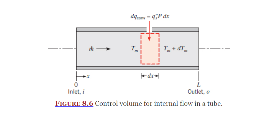
As the flow in completely enclosed, an energy balance can be used to find the mean temperature.
Equation (8.34):
See 7C - 1st Class.
Constant Surface Heat Flux
Covered in Section 8.3.2, analyzing internal flow with constant heat flux is greatly simplified as heat flux becomes independent of location. Equation 8.38 gives convection heat transfer rate:
As shown in 7C - 1st Class and section 8.3.2 we can derive an expression for temperature as a function of location (Equation 8.49):
Idk what Figure 8.7 is, its just "very important" or smth
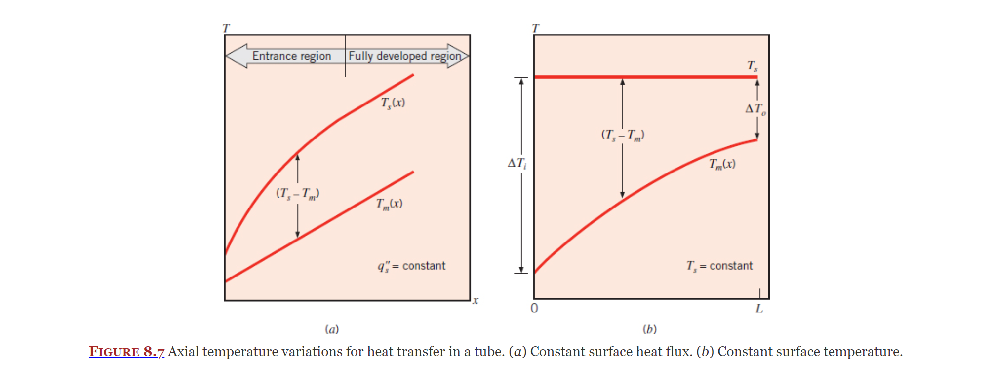
Constant Surface Temperature
Covered in Section 8.3.3, another simplification we can take advantage of is when there is a constant surface temperature.
Equation 8.41b:
Equation 8.42:
Where
Equation 8.45:
See 7C - 1st Class.
Convection heat transfer coefficient is not known
ngl, that sucks
External Flow
Chapter 7
Depending on your problem you can apply various models:
Cylinder in Cross Flow
Section 7.4
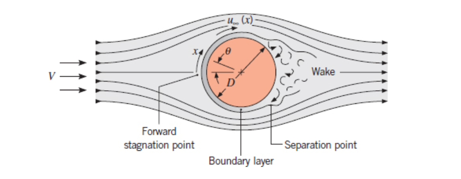
The Hilpert Correlation (Equation 7.52):
Constants
Diameter is used as the characteristic length.
Flow around a Sphere
Section 7.5
Stokes' Law (Equation 7.55):
Where
Equation 7.56:
Where
Equation 7.57:
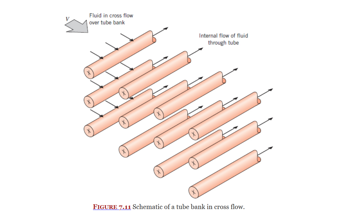
Flow Across Banks of Tubes
Section 7.6
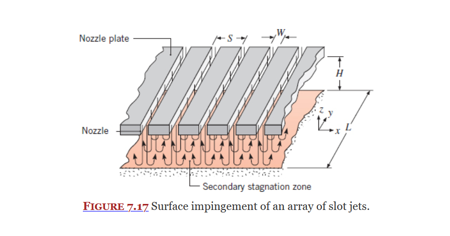
Impinging Jets
Section 7.7
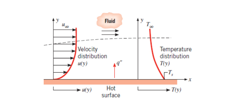
Flat Plate in Parallel Flow
Section 7.2 covers a the convection associated with an isothermal flat plate exposed to flow on one side as shown in the below image.
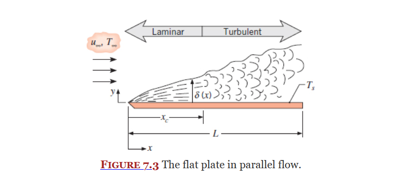
See boundary layers, specifically thermal boundary layers.
Using the similarity transformation on the boundary layer equations, the following equations for continuity, momentum, and energy can be found:
Continuity (Eq. 7.4):
Momentum (Eq. 7.5):
Where
Energy (Eq. 7.6):
Where
See ME3304 S24 Lecture Note (3) Convection and Example 7.1 for more information.
Laminar Flow over an Isothermal Plate
Section 7.2.1
Equation 7.29:
Where
Equation 7.30 (temperature):
Where
Equation 7.31 (mass):
Where
Turbulent Flow over an Isothermal Plate
Section 7.2.2
Equation 7.34:
Where
Velocity boundary layer thickness (Equation 7.35):
Equation 7.36 (temperature):
Where
Equation 7.37 (mass):
Where
Mixed Boundary Layer Conditions
Section 7.2.3
Equation 7.38:
Where
Equation 7.40:
Where
Equation 7.41:
Where
Other conditions
Section 7.2.4 covers a unheated starting length
Section 7.2.5 covers Flat Plates with Constant Heat Flux