Convection

Convection is heat transfer from a solid to a liquid or vise-versa. It is driven by diffusion.

It is given by the following equation:

Where is heat flux, is the convection heat transfer coefficient and is the temperature of the fluid.

Fluid Flow

Chapter 6 reviews convection in depth, fluid flow concepts are heavily involved in this chapter.

convection

Nodal Network

Nodal network is an approximation method to analyze heat transfer in two dimensions (3D will be covered later). They are coved in section 4.4 of the textbook.

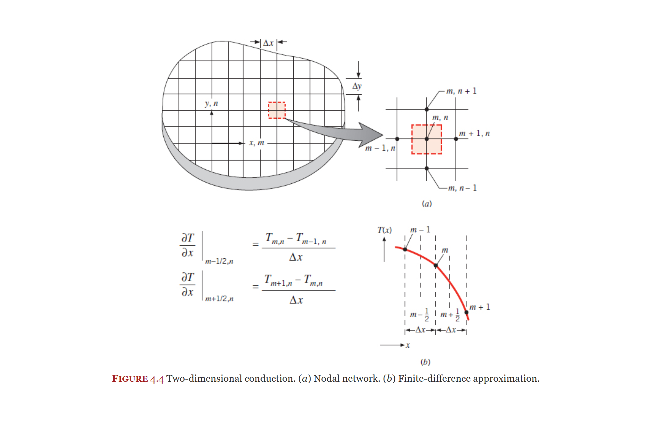
The item you want to analyze is sectioned into nodes (an interior node is shown below), from there the heat transfer rate into and out of the node is balanced.

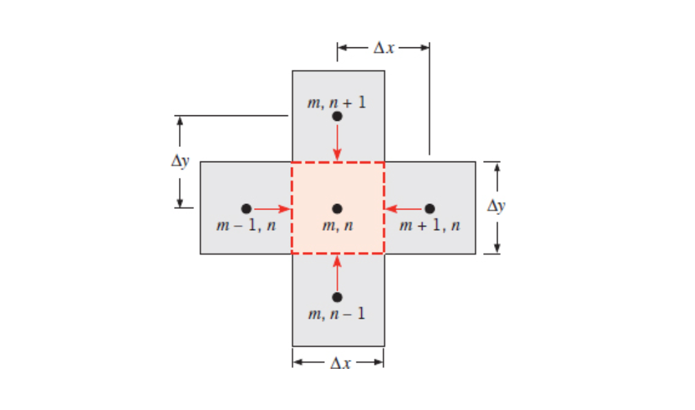
All flows into/out of the node are drawn going into the node (negative heat transfer rates are used to show flows out of the node). From here the heat rate balance can be reduced significantly. See 5A - Class 2 - Finite Difference for an example derivation.

Table of Nodal Finite Difference Equations contains reduced equations for common 2D node conditions.

nodal-network

Finite Difference Analysis

Finite Difference Analysis, also known as finite-element or boundary-element, is a method of analysis that use finite values rather than the continuous ones of other methods.

It is an approximation rather than an exact result.

This method makes use of a nodal network to break a solid up into finite elements.

See the following for examples and more information:

https://youtu.be/LJPSRp0ZeJo?si=xxi1pez7RIWPzSsM

finite-difference-analysis

Heat & Mass Transfer

Used to analyze energy transfer in the form of heat.

Energy and Heat Flow

Heat Flows from hot to cold, we call this heat-transfer-rate.

Heat can flow via 3 methods.

Measurements of Heat

Regardless of how the heat is bring transferred we have to be able to measure it.

Conduction with Heat Generation

This section covers how to analyze conduction problems that include a heat generating solid. It is coved in Section 3.5 of the textbook.

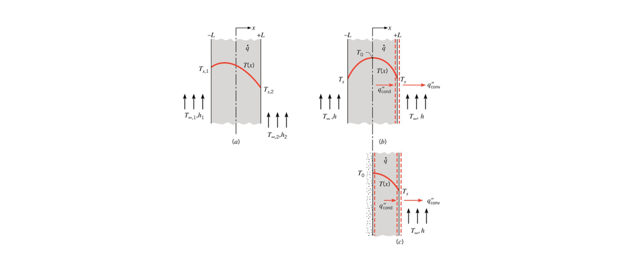
Equation 3.44:

Yields the general solution (Equation 3.45):

Equation 3.46:

Where is half the width of the heat-generation solid, is the surface temperature on the hotter side of the heat generated solid, is the lower temperature, and is the thermal conductivity coefficient.

You cannot use thermal circuit resistance to find a temperature within a heat generating solid.

conduction-with-heat-generation

Volumetric Heat Generation

For materials that generate heat (like nuclear fuel) this is used to measure the amount of heat they generate.

As more mass is added, more heat is generated. Thus this is a function of volume of the heat-generating material.

If you know the width of the heat generating solid () you can convert to heat flux:

volumetric-heat-generation

Conduction

Conduction is the transfer of heat through collisions between atoms/molecules and the diffusion of atoms/molecules of high energy. It is mainly defined by Fourier's Law.

It can occur inside a fluid or a solid. See ME3304 S24 Lecture Note (1) Introduction for more info.

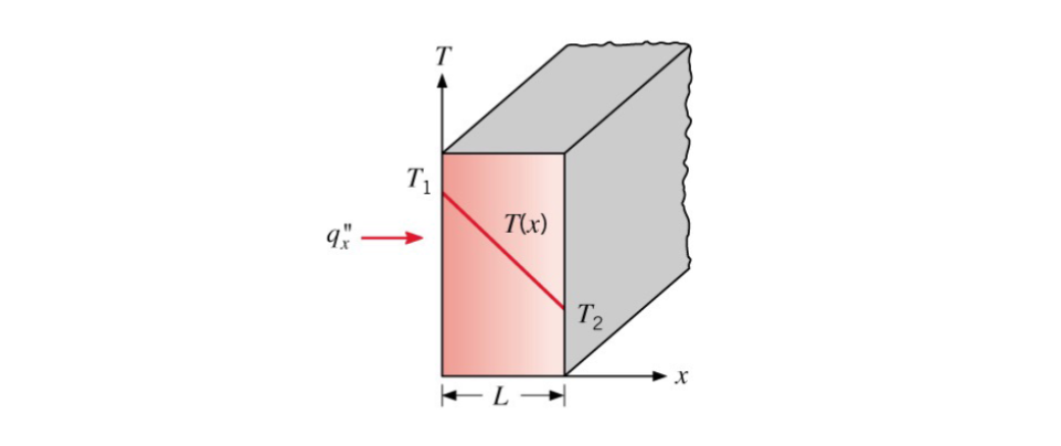
One Dimensional

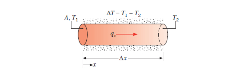
For one-dimensional (x direction only), steady-state, heat diffusion we find that depends on the temperature difference across the solid, the area perpendicular to the flow - , and a material property (which we will call for now).

Thus we can calculate the heat transfer rate as the following:

Again, is a material property referred to as the thermal conductivity coefficient. The minus sign is due to heat always being transferred from hot to cold.

We call the temperature gradient.

We can convert this to heat flux by moving the area over.

Two Dimensional

See finite-difference-analysis

With Heat Generation

See conduction-with-heat-generation

conduction

Semi Infinite Solid

A method that considers space and time.

- Dr. Paul

In contrast to lumped capacitance method which only works on problems that are a function of time, semi-infinite solid method works on problems that are a function of both location and time.

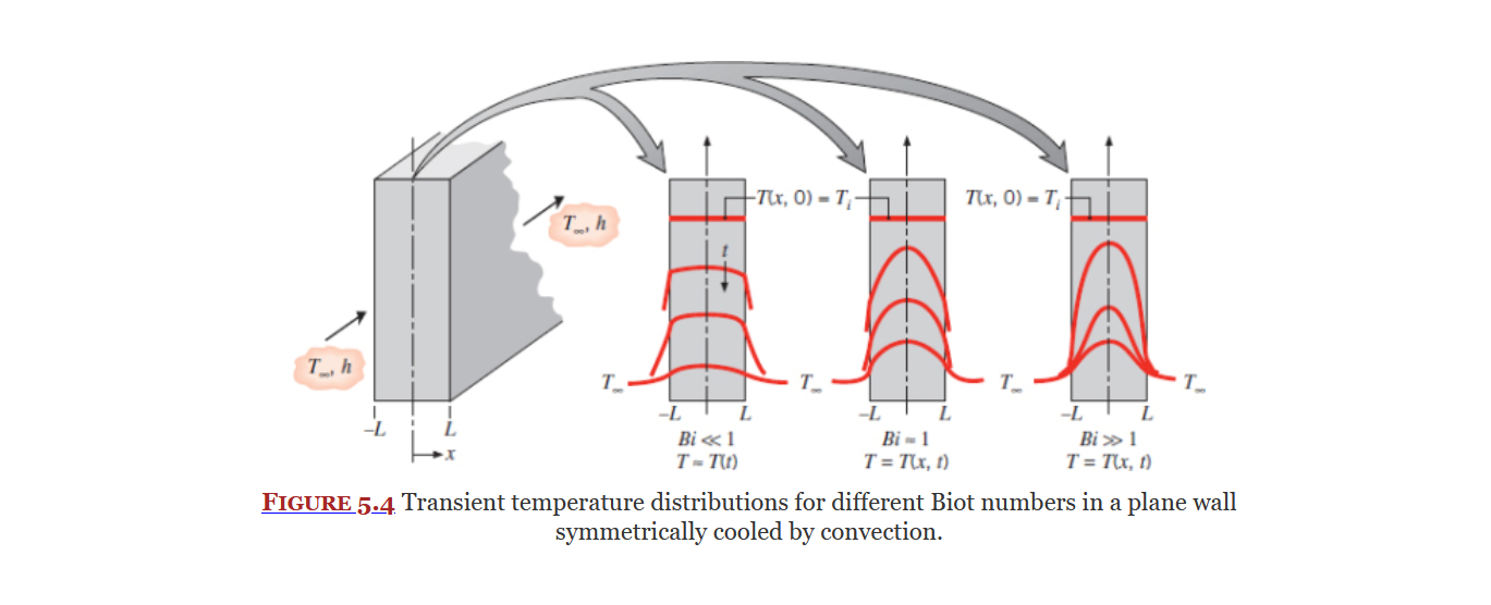
Semi-Infinite Solid is an analysis method that uses a solid that is of infinite size in all but one direction. It is used to analyze temperature of an object over time.

This method yields an analytical solution rather than an approximation, although you are still making an approximation in the fact that infinite solids do not exist. Unlike the lumped capacitance method it can be used where there is a temperature gradient across the solid we are analyzing (the biot number is not very small).

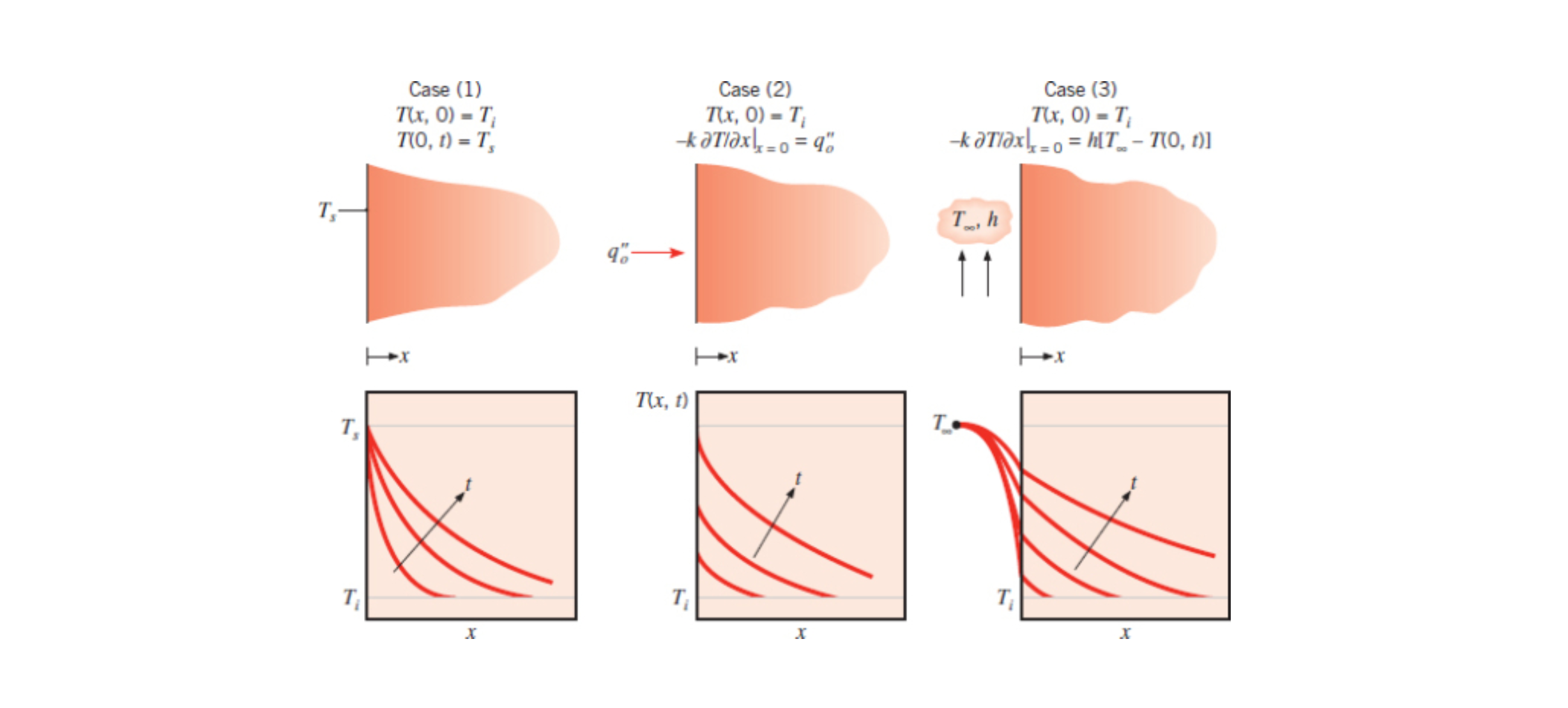
Below are example transient temperature distribution for constant surface temperature (1), constant surface heat flux (2), and surface convection (3).

See Section 5.7, 6E - Class 2, 7A - 2nd Class, and 7C - 2nd Class.

Temperature distribution

The derivation for the following equations (and what the error function is and where it came from) can be found in 7A - 2nd Class.

Equation 5.60:

Where is the similarity variable, is the gaussian error function. Under various conditions equation 5.60 reduces to the following equations.

Case 1 Constant Surface Temperature (Eq. 5.61):

Case 2 Constant Surface Heat Flux (Eq. 5.62):

Case 3 Surface Convection (Eq. 5.63):

Where is the complementary error function, is the thermal diffusivity, is the thermal conductivity coefficient, and is the convection heat transfer coefficient.

Python

Equation 5.63 (Case 3 above):

def caseThree(T, Ti, Too, x, alpha, t, h, k):
  coeffOne = erfc(x/(2*sqrt(alpha * t)))
  coeffTwo = exp(((h*x)/k) + ((h**2 * alpha*t)/k**2))
  coeffThr = erfc((x/2*sqrt(alpha*t)) + ((h*sqrt(alpha*t))/k))
  coeffFou = (T-Ti)/(Too-Ti)

  return coeffOne - coeffTwo * coeffThr - coeffFou

semi-infinite-solid

Heat Flux

Heat flux is heat transfer though a surface. It is perpendicular to the surface it is traveling through.

You can relate heat flux to heat transfer rate using the area of the surface () it is flowing through.

When working with one-dimensional convection and under steady-state conditions we can define heat flux as the following.

fouriers-law

heat-flux

Heat Transfer Rate

Heat transfer rate is the rate of energy transferred between objects via heat. It has units of watts.

When working with thermal circuits heat transfer rate is considered to be current.

heat-transfer-rate

Thermal Diffusivity

Thermal Diffusivity is the diffusion coefficient for heat. Just like there is a diffusion coefficient for momentum, etc.

- Dr. Paul

Thermal diffusivity, , is the ratio between thermal conductivity, , and heat capacity, .

Page 58 of the textbook (Section 2.2.2).

thermal-diffusivity

Fourier Number

The Fourier Number is dimensionless time and is used with the biot number to characterize transient conduction problems. It is defined in equation 5.12 (Section 5.2) as the following:

Where is thermal diffusivity and is characteristic length.

fourier-number

Lumped Capacitance Method

Lumped Capacitance really means that heat transfer is a function of time only.

- Dr. Paul

Lumped Capacitance Method is a continuation of the ideas laid down in thermal circuits. As the name suggests we now have a thermal capacitance, .

This method is an approximation and it only works is there is no temperature gradient across the object. This can be quantified by checking to make sure the biot number is much smaller than 1. See ME3304 S24 Lecture Note (2) Conduction.

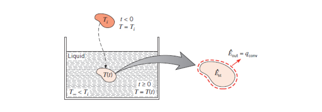
Given a solid of a high temperature that is in an environment that rapidly changes temperature (for example heat treating metal) we imagine that the solid is a capacitor (or battery). As soon as our solid changes environment it will start to discharge its energy as heat.

Equation 5.4 (temperature difference):

Equation 5.5:

Where is density, is volume, is specific heat, is convection heat transfer coefficient, is cross-sectional area, and is time. The component in front of the natural log () is used frequently and is called the thermal time constant.

Equation 5.6:

Where and are the convection thermal resistance and and are the lumped capacitance coefficient.

Relating to thermocouple somehow.

An example of a problem using this method can be found in ME3304 Conduction Previous Test Solution.

Allows you to write energy-stored as the following?

See 6E - Class 2 - Transient Heat Transfer 2024-02-26 17_38_48.

lumped-capacitance-method

Heat Diffusion Equation

Equation 2.19 (below) is the general form of the heat diffusion equation in cartesian coordinates.

Where is volumetric heat generation, is heat capacity.

Cylindrical Coordinates (Eq. 2.26 - Pg. 65)::

Spherical Coordinates (Eq. 2.29 - Pg. 67):

heat-diffusion-equation

Biot Number

Biot Number (Eq. 5.9) is a dimensionless parameter. It is a measure of how dramatic the temperature difference across a solid is in comparison to the temperature difference across the boundary undergoing convection.

Where is the convection heat transfer coefficient, is the characteristic length, and is the thermal conductivity coefficient.

Section 5.2 goes says the following:

Biot number provides a measure of the temperature drop in the solid relative to the temperature difference between the solid's surface and the fluid.

From Equation 5.9, it is also evident that the Biot number may be interpreted as a ratio of thermal resistances.

In particular, if Bi ≪ 1, the resistance to conduction within the solid is much less than the resistance to convection across the fluid boundary layer.

It is used in the lumped capacitance method as well as to tell if the fin approximation can be used... I think, idk.

and are conduction and convection resistances as given in thermal circuits.

biot-number

Fourier's Law

Fourier's Law essentially states that heat flux is always normal to a cross sectional area of constant temperature.

Where is heat flux, is thermal conductivity coefficient, is temperature, and is time.

See ME3304 S24 Lecture Note (1) Introduction for more information.

fouriers-law

Energy Balance

Heat Transfer lives as a subcategory of thermodynamics and is based off its ideas. Energy balance is one of thermodynamics' defining characteristics and is true for heat transfer.

Starting with the a basic energy balance about a control volume we have:

Where is the rate of energy in and is the rate of energy out.

We can develop this further by accounting for energy stored within a control-volume and energy generated by a control volume using the following equation:

See Section 1.3 of the textbook for more information.

This concept is applied to systems using conduction by the heat diffusion equation.

energy-balance

Specific Heat

Specific heat is a measure of how much energy is required to raise a mass by one degree. See below for units.

Specific Heat has units of joules per kilogram kelvin in the metric system. Water has a specific heat of 4181 J/kgK. Therefor 4181 Joules are required to heat up one kilogram of water by one degree Kelvin.

specific-heat

Thermal Capacitance

Built off the idea laid down in thermal circuits, Thermal Capacitance is essentially the idea of electrical capacitance applied to heat. That is to say it is a measure of a materials ability to store heat. It is the driving idea lumped capacitance method.

Where is density, is the volume of your solid (or control volume), and is the specific heat of the material.

Thermal capacitance is covered in section 5.1 of the textbook (page 192).

thermal-capacitance

Thermal Circuits

In many cases heat flow can be analyzed using thermal 'circuits'. When using this approach heat transfer rate becomes current, temperature difference becomes voltage, and resistance is the material's resistance to the heat flow.

Thermal circuits are covered in chapter 3.

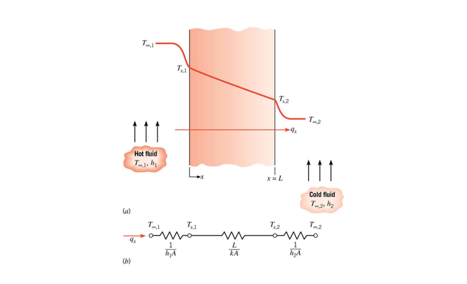
Resistance for conduction:

Where is heat transfer rate in the x direction, is the thermal conductivity coefficient, and is the cross-sectional area (see also Fourier's Law).

Resistance for convection:

Where is convection heat transfer coefficient and is the temperature of the fluid.

Contact Resistance

Section 3.1.4

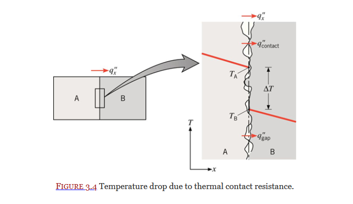
Equation 3.20:

Thermal Capacitance

Thermal capacitance is an idea that builds upon the foundations laid down in thermal circuits. It is explained in its own page.

thermal-circuits

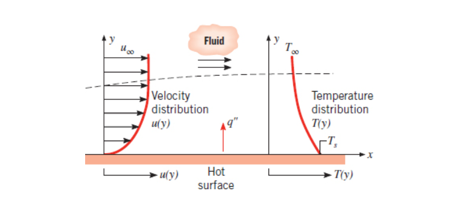
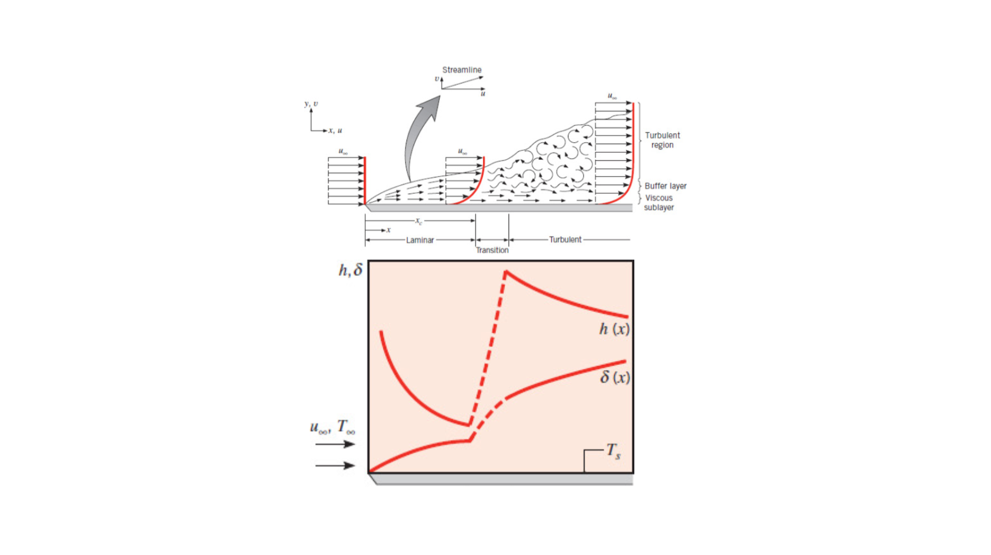
Thermal Boundary Layer

The thermal boundary layer is a fluid boundary layer that is measures the temperature of a fluid as it flows over a surface. The concentration boundary layer is essentially the same thing but it measures mass instead.

Heavily related to velocity boundary layer.

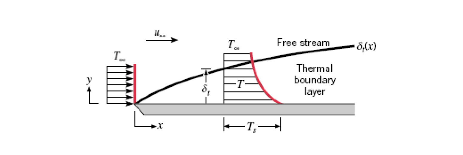
The thermal boundary layer thickness, , increases the further it is down the flow direction.

Heat flux given by the following:

Using this we can find an expression for the convection heat transfer coefficient. If is greater than then:

Then plugging this into our equation for heat flux we get:

See ME3304 S24 Lecture Note (3) Convection for more info.

Equation 6.14:

ME3304 S24 Lecture Note (3) Convection - Page 10

The derivation of Equation 6.14 is shown in 9A - 2nd Class.

thermal-boundary-layer

Internal Flow

Chapter 8

Internal fluid flow is fluid flow that occurs within a pipe or other container.

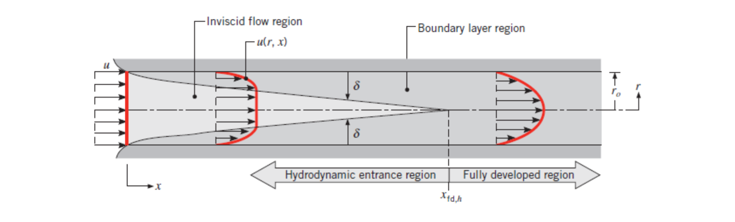
If the flow is laminar (ie. in the fully developed region) the velocity profile is parabolic. See entry-region for how to calculate the distance at which the fully developed region starts.

When dealing with turbulent flow it becomes extremely difficult to find the temperature gradient so instead we use the mean temperature (or mixed bulk temperature).

For internal flow the characteristic length is known has hydraulic diameter.

Mass Flow Rate (Equation 8.5):

Where is density, is velocity, and is cross-sectional area.

See Chapter 8 and ME3304 S24 Lecture Note (3) Convection for more info.

Energy Balance

Section 8.3

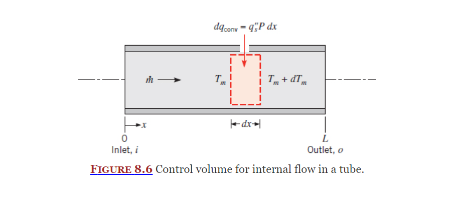
As the flow in completely enclosed, an energy balance can be used to find the mean temperature.

Equation (8.34):

See 7C - 1st Class.

Constant Surface Heat Flux

Covered in Section 8.3.2, analyzing internal flow with constant heat flux is greatly simplified as heat flux becomes independent of location. Equation 8.38 gives convection heat transfer rate:

As shown in 7C - 1st Class and section 8.3.2 we can derive an expression for temperature as a function of location (Equation 8.49):

Idk what Figure 8.7 is, its just "very important" or smth

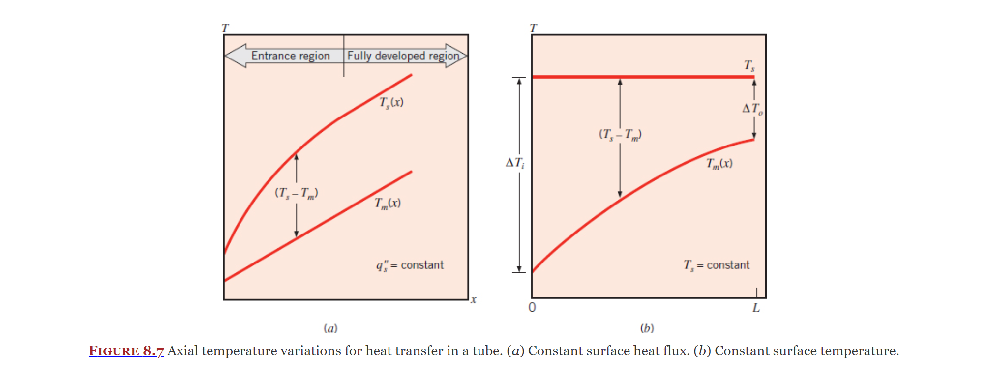
Constant Surface Temperature

Covered in Section 8.3.3, another simplification we can take advantage of is when there is a constant surface temperature.

Equation 8.41b:

Equation 8.42:

Where is the average convection heat transfer coefficient

Equation 8.45:

See 7C - 1st Class.

internal-flow

Flow around a Sphere

Section 7.5

Stokes' Law (Equation 7.55):

Where is drag coefficient.

Equation 7.56:

Where is dynamic viscosity.

Equation 7.57:

flow-around-a-sphere

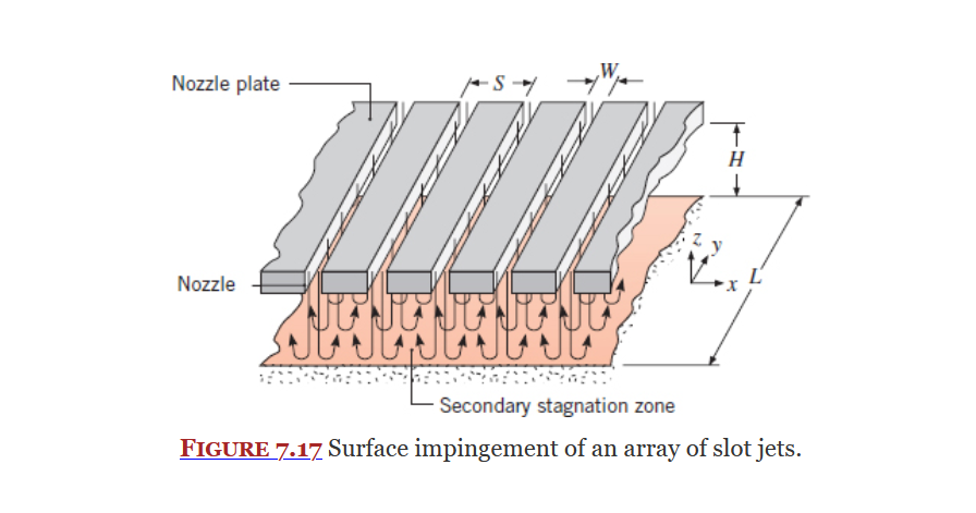
Impinging Jets

Section 7.7

impinging-jets

Laminar Flow

A fluid-flow concept.

laminar-boundary-layer

laminar-flow

Laminar Boundary Layer

In contrast to turbulent-boundary-layer.

You can find the point at which flow becomes turbulent using the critical reynolds number.

fluid-flow
laminar-flow

velocity-boundary-layer
thermal-boundary-layer

See ME3304 S24 Lecture Note (3) Convection for more info.

laminar-boundary-layer

Critical Reynolds Number

Covered in Section 6.3.1, the critical Reynold's Number is the Reynold's number at which the boundary layer flow transitions from laminar to turbulent.

The Critical Reynold's Number is defined in equation 6.24:

Where is the distance at which the flow transitions from laminar to turbulent, is density, is dynamic-viscosity.

is a typical value for Critical Reynolds Number for external flow.

See 9A - 2nd Class for more information.

critical-reynolds-number

Reynolds Number

A dimensionless parameter that is commonly used to characterize fluid flow, generally turbulent flow.

Where is density, is velocity, is characteristic length, is dynamic viscosity, and is kinematic viscosity.

The Critical Reynold's Number is used to find the point in a boundary layer at which the flow transitions from laminar to turbulent.

ME3304 S24 Lecture Note (3) Convection

reynolds-number

Dimensional Analysis

A fluid-flow concept, relies heavily on the use of dimensionless parameters.

See:

dimensional-analysis

Dimensionless Parameters

Parameters that have no unit of measurement, commonly used in dimensional analysis for analyzing fluid flow.

All dimensionless parameters are just ratios of one thing to another.

- Dr. Paul (paraphrased)

In heat transfer many dimensionless parameters use the star notation.

Table of Heat Transfer Dimensionless Parameters

Table 6.2 is a list of dimensionless parameters applicable to heat transfer.

Group	Definition	Interpretation
Biot Number (Bi)	$\frac{h L}{k_{s}}$	Ratio of the internal thermal resistance of a solid to the boundary layer thermal resistance
Mass transfer Biot number (Bi_m)	$\frac{h_{m} L}{D_{AB}}$	Ratio of the internal species transfer resistance to the boundary layer species transfer resistance
Bond number (Bo)	$\frac{g (ρ_{l} - ρ_{υ}) L^{2}}{σ}$	Ratio of gravitational and surface tension forces
Coefficient of friction (C_f)	$\frac{τ_{s}}{ρ V^{2} / 2}$	Dimensionless surface shear stress
Eckert number (Ec)	$\frac{V^{2}}{c_{p} (T_{s} - T_{\infty})}$	Kinetic energy of the flow relative to the boundary layer enthalpy difference
Fourier number (Fo)	$\frac{α t}{L^{2}}$	Ratio of the heat conduction rate to the rate of thermal energy storage in a solid. Dimensionless time
Mass transfer Fourier number (Fo_m)	$\frac{D_{{AB}^{t}}}{L^{2}}$	Ratio of the species diffusion rate to the rate of species storage. Dimensionless time
Friction factor (f)	$\frac{Δ p}{(L / D) (ρ u_{m}^{2} / 2)}$	Dimensionless pressure drop for internal flow
Grashof number (Gr_L)	$\frac{g β (T_{s} - T_{\infty}) L^{3}}{ν^{2}}$	Measure of the ratio of buoyancy forces to viscous forces
Colburn j factor (j_H)	St Pr^2/3	Dimensionless heat transfer coefficient
Colburn j factor (j_m)	St_m Sc^2/3	Dimensionless mass transfer coefficient
Jakob number (Ja)	$\frac{c_{p} (T_{s} - T_{sat})}{h_{f g}}$	Ratio of sensible to latent energy absorbed during liquid–vapor phase change
Lewis number (Le)	$\frac{α}{D_{AB}}$	Ratio of the thermal and mass diffusivities
Mach number (Ma)	$\frac{V}{a}$	Ratio of velocity to speed of sound
Nusselt number (Nu_L)	$\frac{h L}{k_{f}}$	Ratio of convection to pure conduction heat transfer
Peclet number (Pe_L)	$\frac{V L}{α} = {Re}_{L} \Pr$	Ratio of advection to conduction heat transfer rates
Prandtl number (Pr)	$\frac{c_{p} μ}{k} = \frac{ν}{α}$	Ratio of the momentum and thermal diffusivities
Reynolds number (Re_L)	$\frac{V L}{ν}$	Ratio of the inertia and viscous forces
Schmidt number (Sc)	$\frac{ν}{D_{AB}}$	Ratio of the momentum and mass diffusivities
Sherwood Number (Sh_L)	$\frac{h_{m} L}{D_{AB}}$	Ratio of convection to pure diffusion mass transfer
Stanton number (St)	$\frac{h}{ρ V c_{p}} = \frac{{Nu}_{L}}{{Re}_{L} \Pr}$	Modified Nusselt number
Mass Transfer Stanton number (St_m)	$\frac{h_{m}}{V} = \frac{{Sh}_{L}}{{Re}_{L} Sc}$	Modified Sherwood number
Weber number (We)	$\frac{ρ V^{2} L}{σ}$	Ratio of inertia to surface tension forces

dimensionless-parameters

Fully Developed Region

The fully developed region of an internal flow is the point at the boundary-layer merges with itself. See photo below:

See How to calculate entry length.

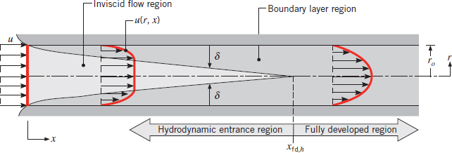
Section 8.1.1

fully-developed-region

Flow in Noncircular Tubes

Section 8.6

flow-in-noncircular-tubes

Concentration Boundary Layer

The concentration boundary layer is like thermal boundary layer but if the temperature was instead mass.

Essentially measures density?

9A - 2nd Class

concentration-boundary-layer

Reynolds Analogy

The following equation (Equation 6.69) is known as the Reynolds Analogy. It allows other parameters to be found if the velocity is known and vise versa. It consists of dimensionless parameters.

Where is Friction Coefficient, is Stanton number, and is the Mass Transfer Stanton number.

This analogy is further expanded by the Modified Reynolds analogy (Eq. 6.70):

And the Chilton-Colburn analogy:

See Section 6.7.3 (page 298) and ME3304 S24 Lecture Note (3) Convection.

The following is from lecture 7A, not sure what it means or if its true

reynolds-analogy

Flat Plate in Parallel Flow

Section 7.2 covers a the convection associated with an isothermal flat plate exposed to flow on one side as shown in the below image.

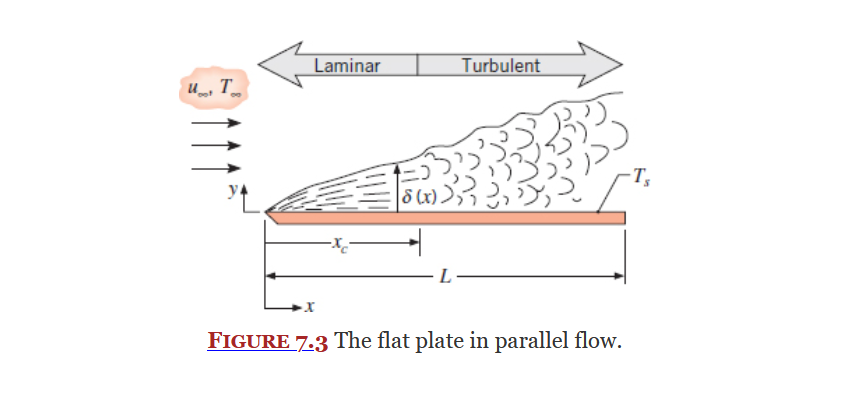
See boundary layers, specifically thermal boundary layers.

Using the similarity transformation on the boundary layer equations, the following equations for continuity, momentum, and energy can be found:

Continuity (Eq. 7.4):

Momentum (Eq. 7.5):

Where is kinematic viscosity.

Energy (Eq. 7.6):

Where is thermal diffusivity.

See ME3304 S24 Lecture Note (3) Convection and Example 7.1 for more information.

Laminar Flow over an Isothermal Plate

Section 7.2.1

Equation 7.29:

Where is the friction-coefficient and is reynolds-number.

Equation 7.30 (temperature):

Where is the Nusselt Number, is the average convection heat transfer coefficient, and is the Prandtl Number.

Equation 7.31 (mass):

Where is the Sherwood number, is the average convection mass transfer coefficient, and is the Schmidt number.

Turbulent Flow over an Isothermal Plate

Section 7.2.2

Equation 7.34:

Where is the friction coefficient and is the Reynolds number.

Velocity boundary layer thickness (Equation 7.35):

Equation 7.36 (temperature):

Where is the Nusselt number, is the Stanton number, and is the Prandtl number.

Equation 7.37 (mass):

Where is the Sherwood number, is the Stanton number, and is the Schmidt number.

Mixed Boundary Layer Conditions

Section 7.2.3

Equation 7.38:

Where is the Nusselt number and is the Prandtl number.

Equation 7.40:

Where is the friction coefficient.

Equation 7.41:

Where is the Sherwood number and is the Schmidt number.

Other conditions

Section 7.2.4 covers a unheated starting length
Section 7.2.5 covers Flat Plates with Constant Heat Flux

flat-plate-in-parallel-flow

Laminar Flow in Circular Tubes

Section 8.4 covers laminar flow in circular tubes (internal-flow).

In the fully developed region

Constant Heat Flux (Equation 8.53):

Constant Surface Temperature (Equation 8.55):

The derivation of equations 8.55 and 8.53 can be found in 11A - 2nd Class.

In the entry region

Equation 8.56:

Equation 8.57:

Equation 8.58:

laminar-flow-in-circular-tubes

Entry Region

The entry region is the region before the fully developed region in an internal flow.

How to calculate entry length

Section 8.1.1

If flow is laminar (Equation 8.3):

If flow is turbulent (Equation 8.4):

If --> fully developed turbulent flow.

entry-region

Turbulent Flow in Circular Tubes

Section 8.5

Fully Developed Flow

The Dittus-Boelter equation (Equation 8.60) is valid for small temperature differences:

Where is 0.4 when and 0.3 when .

The derivation for the Dittus-Boelter Correlation can be found in 11A - 2nd Class.

Large Temperature Differences

Equation 8.61:

Smooth tubes

Equation 8.62 is more accurate than 8.61 but only applicable to smooth tubes:

turbulent-flow-in-circular-tubes

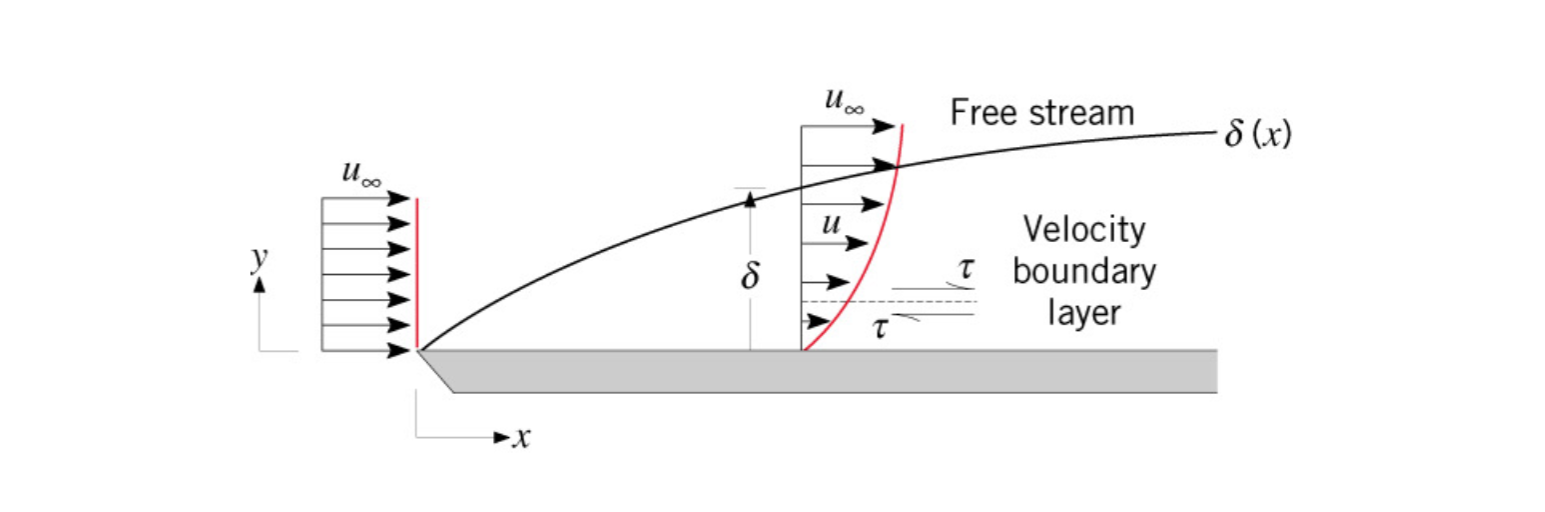
Velocity Boundary Layer

Heavily related to thermal boundary layer.

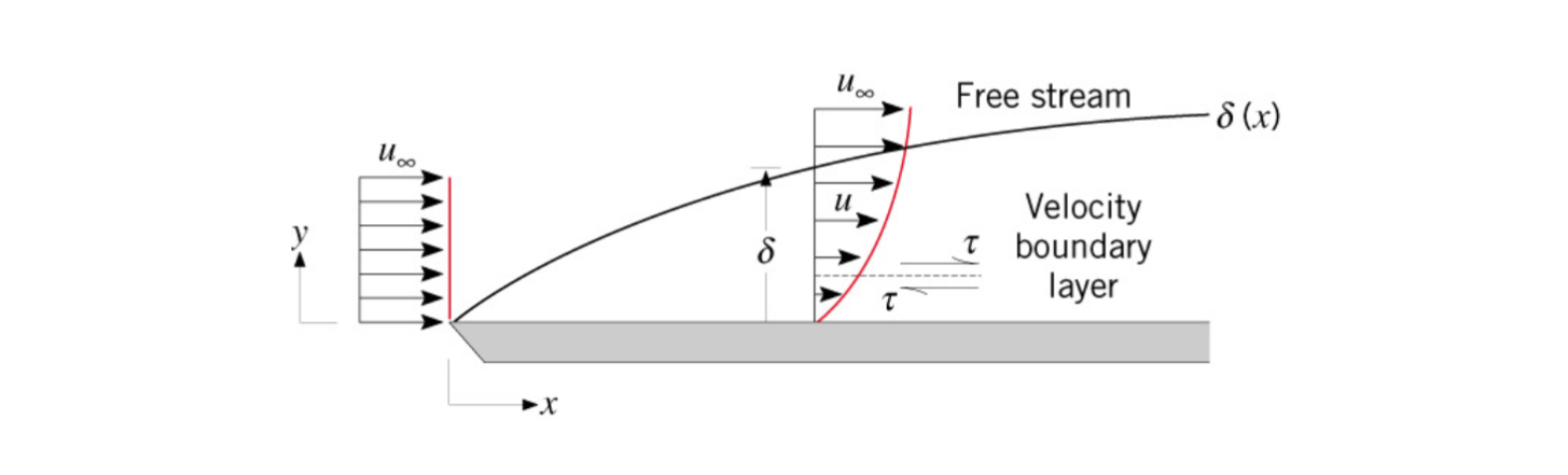
Surface frictional drag may be found using the friction coefficient. (Section 6.1.1)

The edge of the boundary layer is where the fluid it traveling 99% of the free stream velocity.

ME3304 S24 Lecture Note (3) Convection

velocity-boundary-layer

Turbulent Flow

A fluid flow concept.

Everything is more in turbulent, more heat transfer, more drag, etc.
- Dr. Paul

turbulent-boundary-layer

turbulent-flow

Turbulent Boundary Layer

In contrast to laminar-boundary-layer.

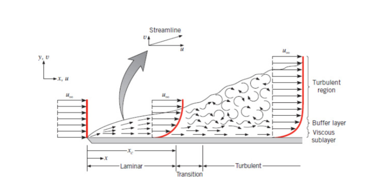
You can find the point at which flow becomes turbulent using the critical reynolds number.

The circular flow within turbulent flow are called eddies.

fluid-flow
turbulent-flow

velocity-boundary-layer
thermal-boundary-layer

See ME3304 S24 Lecture Note (3) Convection for more info.

turbulent-boundary-layer

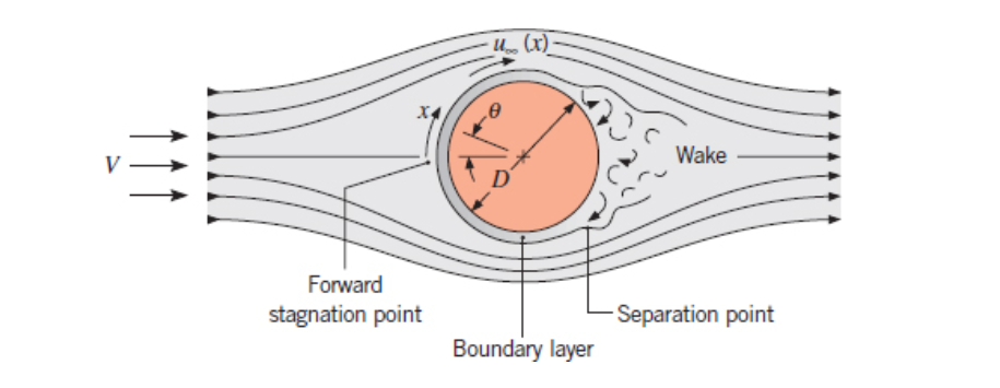
Cylinder in Cross Flow

Section 7.4

The Hilpert Correlation (Equation 7.52):

Constants and are listed in table-7.2. Constants for non-cylindrical geometries can be found in table-7.3.

Diameter is used as the characteristic length.

cylinder-in-cross-flow

External Flow

Chapter 7

Depending on your problem you can apply various models:

external-flow

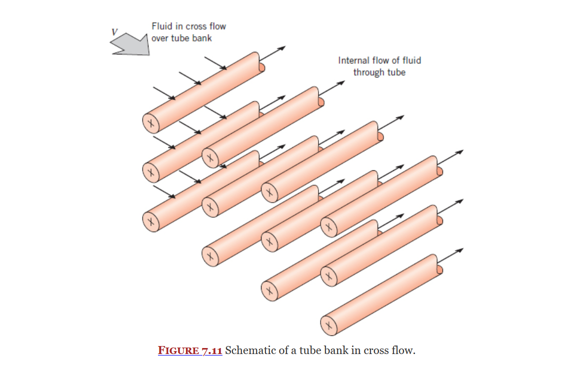
Flow Across Banks of Tubes

Section 7.6

flow-across-banks-of-tubes

Fluid Flow

Fluid flow has a large impact on convection and needs to be accounted for when finding the convection heat transfer coefficient.

The largest two factors that effect convection are:

Where does the flow occur? (externally or internally)
What form does the flow take? (laminar or turbulent)
This can be found out by calculating the reynolds-number and comparing it to the typical critical-reynolds-number.

Flow might be both laminar and turbulent, boundary layers are used to analyze these flows against surfaces. There are three types of boundary layers that are of interest to this class:

Velocity boundary layer measures fluid velocity.
Thermal boundary layer measures temperature.
Concentration boundary layer measures mass.

Fluid Flow makes heavy use of dimensionless parameters.

The Reynolds Analogy is used often to relate parameters in a flow.

fluid-flow

Extended Surfaces (Fins)

Extended Surfaces or Fins are sections of an object that extend out into a fluid used for heat dissipation. They are covered in Section 3.6.

General form of energy dissipation equation for a fin (Eq. 3.66):

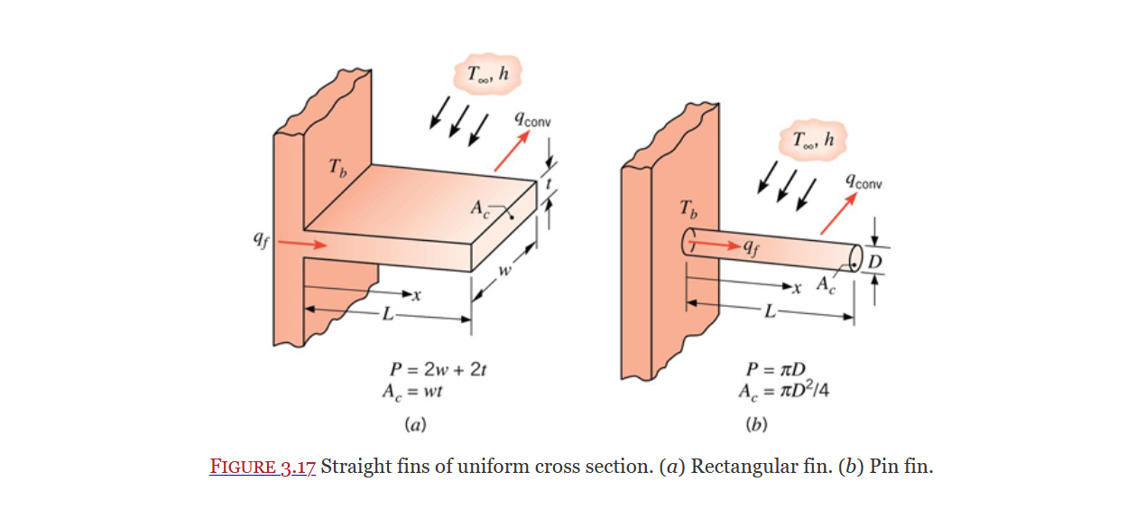
In the above image the cross section does not change along the length of the fin, thus the general equation can be reduced to the following (Eq. 3.67):

The following two definitions (Eq. 3.68 & 3.70):

allow us to reduce our equation (Eq. 3.69):

Now that it is in this form we can find it's general solution to be (Eq. 3.71):

We generally refer to as a temperature difference.

A derivation for a rod fin can be found in 4E - Class 2 - Fins Cont. 2024-02-13 00_10_36

Hyperbolic tribometry functions (namely ) appears frequently. This is due to it's definition:

See extended-surface-equation-table for equations related to extended surfaces.

fin-effectiveness
fin-efficiency

extended-surfaces

Fin Effectiveness

convection-heat-transfer-coefficient
heat-transfer-rate

fin-effectiveness

Fin Efficiency

Where is the heat transfer rate of the fin, is convection heat transfer coefficient, is the total surface area of the fin including the tip, is known as temperature difference.

fin-efficiency

About this chart

Layout

Concepts build as they go down the chart, all ideas aim to build on the three main heat transfer methods. Arrows point from prerequisite information to the concepts they support.

Color Code

White - General Information/Concepts and Topics
Gray/Black - Supporting Concepts, Equations, and Ideas
Red - conduction
Orange - convection
Yellow - radiation
Green - mass transfer
Purple - topics that contain a combination of the above three heat transfer modes
Blue - topics related to fluid flow

Boundary Layer

A boundary is a section of fluid that flows up-against some surface. Typically the velocity is slower closer to the surface, while at some distance away from the surface the velocity is traveling as fast as the rest of the fluid. This concept is called the velocity boundary layer. There are three main boundary layers covered in this course:

Velocity boundary layer as mentioned above.
Thermal boundary layer which is concerned with temperature.
Concentration boundary layer which is concerned with mass.

Boundary layer thickness is denoted as .

There are multiple types of boundary layers, namely velocity boundary layer and thermal boundary layer.

Fluid flow inside a boundary layer can be laminar or turbulent.

See ME3304 S24 Lecture Note (3) Convection for more information.

ME3304 S24 Lecture Note (3) Convection

boundary-layer

Heat Exchanger - Overall Heat Transfer Coefficient

Section 11.2

When this is large you have a lot of heat transfer.

- Dr. Paul

Equation 11.1a:

Where refers to the cold fluid, refers to the hot fluid, is the thermal resistance, is the overall heat transfer coefficient, and is the area of the heat flux.

Equation 11.1b:

Where is the similarity variable? is thermal resistance

heat-exchanger-overall-heat-transfer-coefficient

Heat Exchanger Effectiveness-NTU Method

Section 11.4

The Effectiveness-NTU method is an heat exchanger analysis method like the log-mean temperature analysis method but doesn't require knowing the outlet temperatures.

NTU stands for number of mass transfer units.

After defining heat exchanger effectiveness () the following equations can be made:

Equation 11.20 (Hot fluid):

Equation 11.21 (Cold fluid):

Where subscripts and refer to hot and cold, subscripts and refer to inlet and outlet, is the heat capacity rate, is either or - whichever is smaller, and is temperature.

Table 11.3 and Table 11.4 - Heat Exchanger NTU relations provide relationships between effectiveness and NTU (number of mass transfer units).

ME3304 S24 Lecture Note (6) Heat Exchanger, 12C - 2nd Class.

heat-exchanger-effectiveness-NTU-method

Overall Heat Transfer Coefficient

It's "overall" because it includes more than just convection.

- Dr. Paul

The overall heat transfer coefficient () is defined in chapter 3 by Equation 3.18:

Where is the total thermal resistance and is the area of heat flux (same area used in Fourier's Law).

heat-exchanger-overall-heat-transfer-coefficient

overall-heat-transfer-coefficient

Heat Exchanger Effectiveness

Section 11.4.1

Used in the effectiveness-NTU analysis method.

Defined in equation 11.19 as the ratio of actual heat transfer to the maximum possible heat transfer:

heat-exchanger-effectiveness

Number of Mass Transfer Units

NTU is a dimensionless parameter used in the effectiveness-NTU analysis method.

It is defined on page 508 of the text book, in equations 11.23 and 11.24. Equation 11.24 is listed below:

Where is overall heat transfer coefficient, is area, and is the smaller heat capacity rate (pick from either the hot or the cold fluid in your heat exchanger).

As with all non-dimensional parameters we can think of this as a ratio of two things.

A heat exchanger will be better if this number is larger.

- Dr. Paul

NTU

Log Mean Temperature Difference Analysis

Section 11.3

Log Mean Temperature Difference Analysis is a heat exchanger analysis method that can be used if you know the inlet and outlet temperatures of your hot and cold fluids and one of the mass flow rates. You can then calculate the heat transfer between the fluids and the overall heat transfer coefficient.

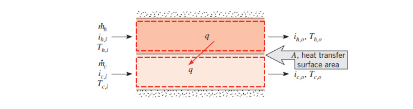
Energy balance of the hot fluid (Equation 11.6a):

Energy balance of the cold fluid (Equation 11.7a):

Where is heat transfer rate, subscript and refer to hot and cold, subscript and refer to inlet and outlet, is enthalpy, and is the mass flow rate.

If the fluids stay in the same phase and you can assume a constant specific heat as they change temperature then you can use temperature instead of enthalpy:

Energy balance of the hot fluid (Equation 11.6b):

Energy balance of the cold fluid (Equation 11.7b):

Where is specific-heat and is temperature.

See ME3304 S24 Lecture Note (6) Heat Exchanger and 12A - 2nd Class for more information.

See ME3304 S24 Lecture Note (6) Heat Exchanger, page 21 for information about how to determine the mean temperature.

If you need to find the heat-exchanger-overall-heat-transfer-coefficient you can use equation 11.14:

Where is area and is log mean temperature difference.

Log Mean Temperature Difference is defined in equation 11.15:

and for a parallel flow heat exchanger are defined as the following:

For a counter flow heat exchanger they are defined by equation 11.17:

Special Operating Conditions

Section 11.3.3

log-mean-temp-diff-analysis

Parallel-Flow Heat Exchanger

Section 11.3.1 - heat-exchangers

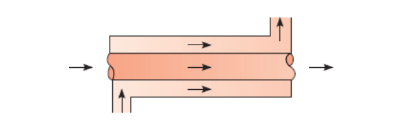
Parallel-flow is more efficient than counter-flow for shorter heat-exchangers.

parallel-flow-heat-exchanger

Counter Flow Heat Exchanger

Section 11.3.2 - heat-exchangers

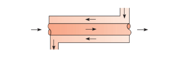
Counter-flow is more efficient than parallel-flow provided that the heat exchanger is long enough.

ME3304 S24 Lecture Note (6) Heat Exchanger

counter-flow-heat-exchanger

Cross Flow Heat Exchanger

heat-exchangers

cross-flow-heat-exchanger

Shell-Tube Heat Exchanger

heat-exchangers

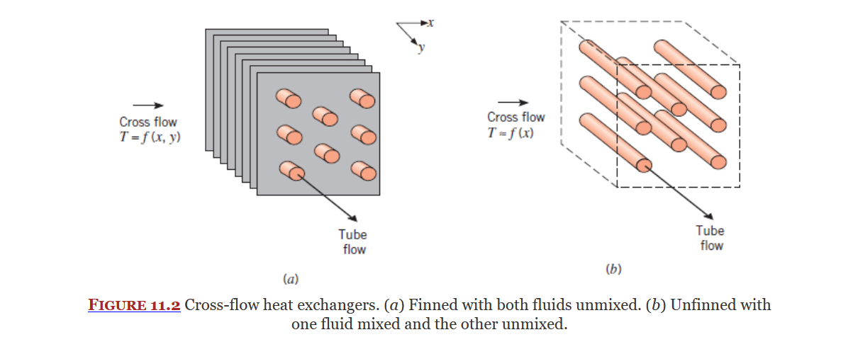
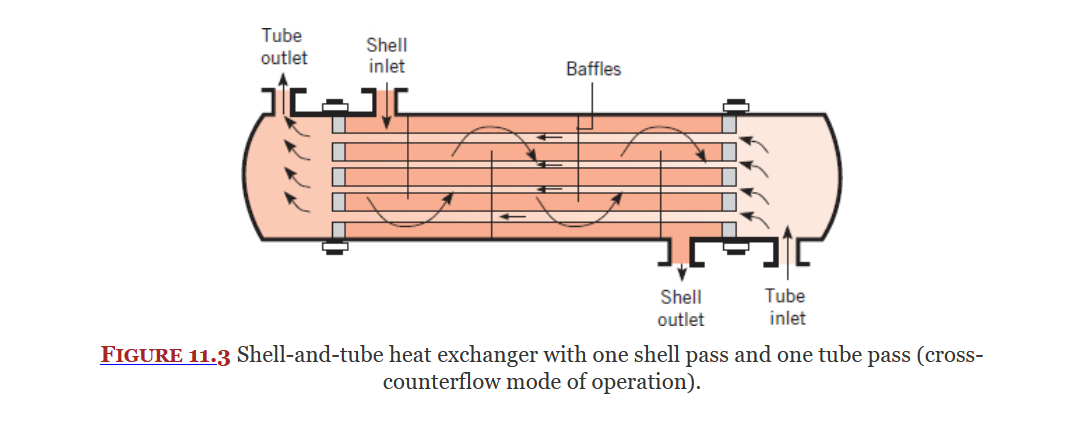
shell-tube-heat-exchanger

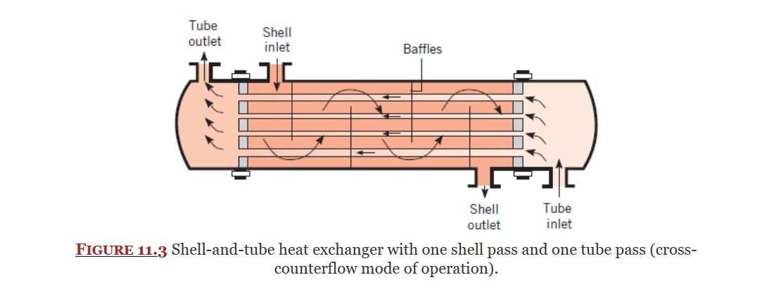
Types of Heat Exchangers

Heat Capacity Rate

A measure of how much heat energy a substance than hold/take on?

Where is mass flow rate and is specific heat.

Defined in equations 11.10 and 11.11.

heat-capacity-rate

Analysis Methods

Heat Exchangers

Covered in Chapter 11, Heat Exchangers are used to transfer heat between two fluids.

There are multiple types of heat exchangers:

Heat Transfer Analysis Methods:

log mean temperature difference analysis - if you know the inlet and outlet temps and mass flow rate of either fluid
effectiveness-NTU analysis method

See ME3304 S24 Lecture Note (6) Heat Exchanger for more information.

The following are notes from Dr. Paul's section covering heat exchangers:

heat-exchangers

Mass Flow Rate

Equation 8.5:

or the fluids version:

Where V is velocity and A is cross-sectional area.

mass-flow-rate

Mass Transfer

Mass transfer is driven by concentration () difference much like heat transfer is driven by a temperature difference.

Species is a term commonly used to refer to some group of mass, often the group is of the same element or chemical.

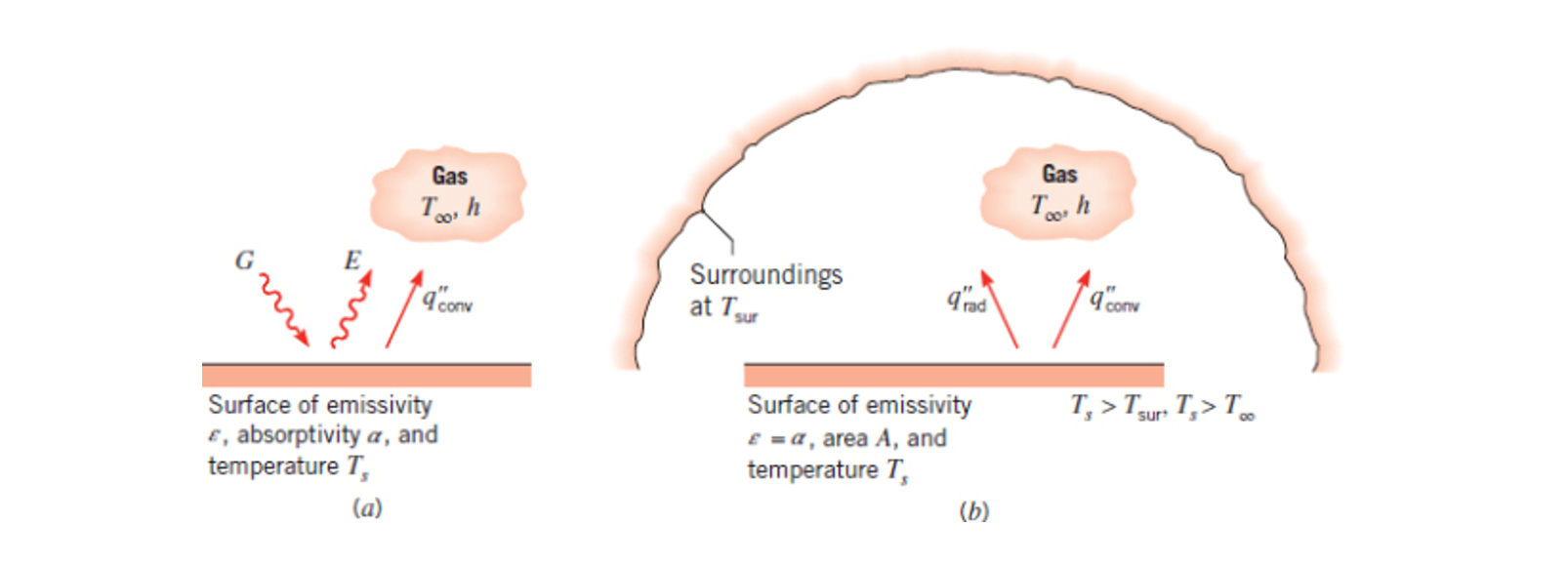
A species molecular weight () is defined by the mass-density () and molecular-concentration ().

mass-transfer

Grey Surface

Covered in Section 12.8, a grey surface is any surface that is not a blackbody, in other words, its emissivity is less than 1.

For a grey body the emissivity is equal to the absorptivity, that is:

A grey surface is a closer approximation to real surfaces but the due to the above correlation it doesn't always match real surfaces.

grey-surface

Reflectivity

Fraction of irradiation reflected.

ME3304 S24 Lecture Note (7) Radiation

reflectivity

Absorptivity

Equation 1.6, the amount of irradiation absorbed.

Equation 12.47:

absorptivity

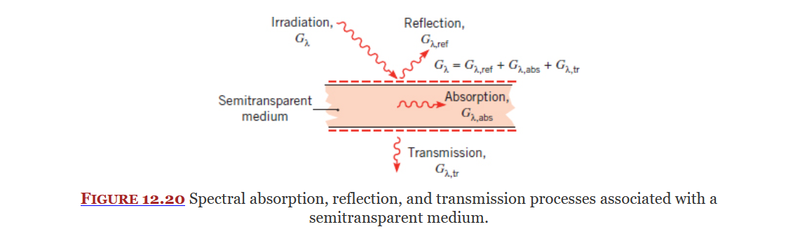
Transmissivity

The fraction of irradiation transmitted through the medium.

transmissivity

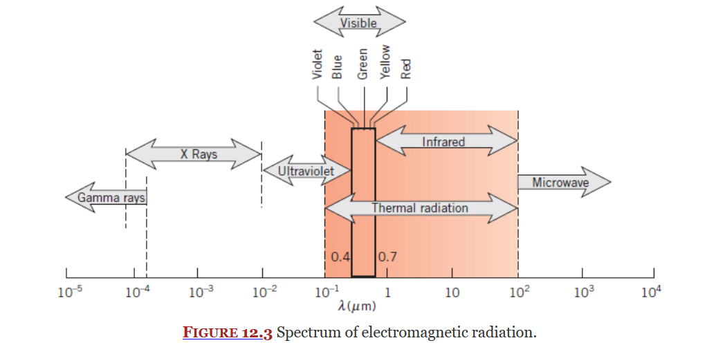
Thermal Radiation

Thermal radiation is a section of the electromagnetic radiation spectrum. It incudes some of ultraviolet, all of visible light, and all of infrared. Thermal radiation is an electromagnetic wave.

See ME3304 S24 Lecture Note (7) Radiation and Section 12.1 for more information.

thermal-radiation

Radiation Heat Fluxes

Covered in Section 12.2, and listed out in table 12.1, the four radiation heat fluxes are the components that make up the energy transfer by way of radiation.

These components are indeed heat fluxes and as such have units of . Listed out they are:

emissive power, , is the radiation emitted by a surface.
irradiation, , is the radiation incident on a surface.
radiosity, , is the radiation leaving a surface.
net radiative flux, , is the net radiation leaving a surface.

See ME3304 S24 Lecture Note (7) Radiation for more info.

13E - 2nd Class

radiation-heat-fluxes

Emissive Power

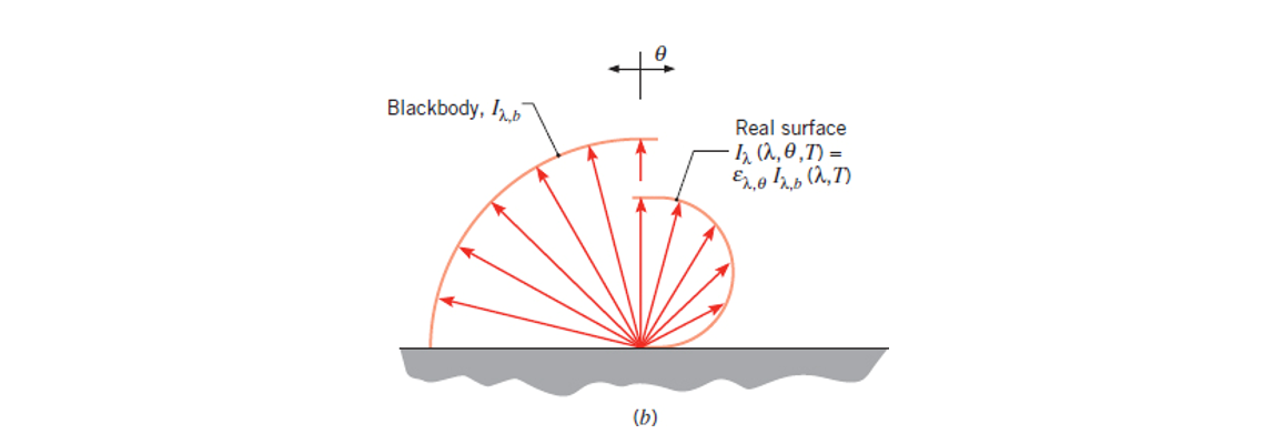
Emissive Power is a radiation heat flux and is represented by . It is a measurement of radiation emitted by a body.

If your object is an ideal radiator it is called a black body, and its radiation is given by Equation 1.4:

Otherwise, if your object is a real surface its radiation is instead given by Equation 1.5:

Where is emissivity, is the Stefan-Boltzmann Constant, and is the absolute temperature of the surface in Kelvin.

Spectral Emissive Power

spectral-intensity

Equation 12.15:

Where and are angles as defined in radiation-intensity and is spectral intensity.

See 14C - 2nd Class for more information.

For a diffuse emitter:

emissive-power

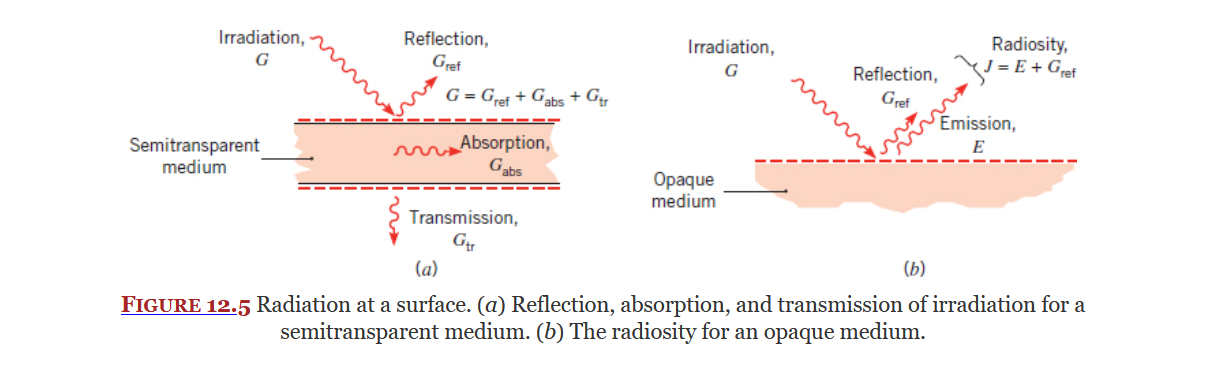
Irradiation

Covered in Section 12.2, Irradiation is the radiation incident (acted upon) on a surface. It is a radiation heat flux represented by and listed in table 12.1.

See ME3304 S24 Lecture Note (7) Radiation and 14A - 2nd Class for more info.

radiation-balance

Components

There are three main components to irradiation.

For most surfaces you can use Equation 12.2:

For an opaque medium there is no transmission so Equation 12.2 becomes 12.3:

See Section 12.2 and ME3304 S24 Lecture Note (7) Radiation for more infomation.

Spectral Irradiation

spectral-intensity

14C - 2nd Class

irradiation

Radiosity

Radiosity is a radiation heat flux, it is represented by (table-12.1).

For an opaque surface:

Where is emissive power, is irradiation, and is reflectivity.

Spectral Radiosity

spectral-intensity

14C - 2nd Class

radiosity

Net Radiative Flux

Listed in table 12.1 as the following:

From ME3304 S24 Lecture Note (7) Radiation, Slide 4:

Where is heat-transfer-rate, is area, is emissivity, is absorptivity, is the emissive power if the object was a blackbody, is irradiation, is the Stefan-Boltzmann-Constant, and is temperature.

net-radiative-flux

Blackbody

Covered in section 12.4, a black body is an object/solid that absorbers all radiation it receives, emits perfectly (it has an emissivity of 1), and emits in all directions (diffuse emitter).

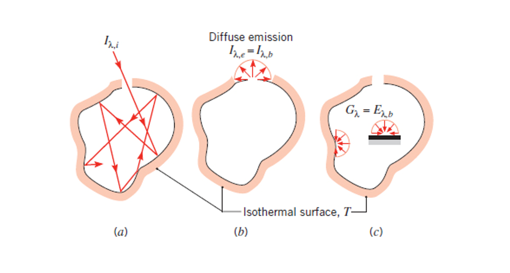
Blackbodies are:

Perfect absorbers ()
Perfect emitters ()
Grey - radiation does not depend on (, ) (they are diffuse)
Emitted radiation is a function of wavelength () and temperature ().

See ME3304 S24 Lecture Note (7) Radiation and 14E - 2nd Class for more information.

Equation 12.29 (blackbody spectral intensity):

See 14E - 2nd Class for details about this equation.

A comparison of a black body to a real surface can be found on Slide 32 of ME3304 S24 Lecture Note (7) Radiation.

blackbody

Emissivity

A material property, defined in Section 12.5, it measures how efficiently a surface emits energy in reference to a black body.

In other words it is the ratio of the radiation emitted by a surface to the radiation emitted by a blackbody of the same temperature.

Used in Equation 1.5 and Example 5.2.

Equation 12.38:

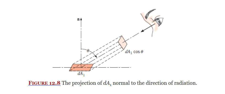
Where is wavelength, and are angles as defined in radiation intensity, is temperature, and is spectral intensity. Subscript refers to blackbody.

emissivity

Radiation Intensity

Section 12.3

radiation + geometryyyyy

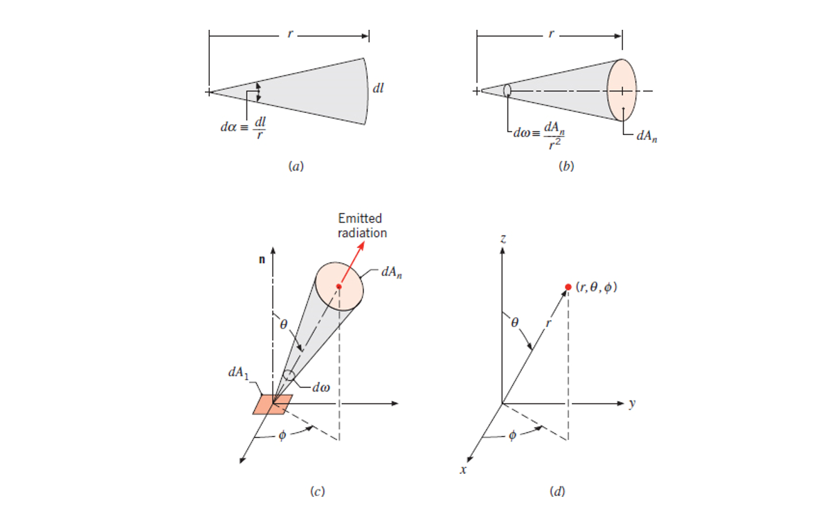
Figure 12.6 - Mathematical definitions (a) Plane angle. (b) Solid angle. (c) Emission of radiation from a differential area into a solid angle subtended by at a point on . (d) The spherical coordinate system.

ME3304 S24 Lecture Note (7) Radiation, 14A - 2nd Class, 14E - 2nd Class

radiation-intensity

Solid Angle

Covered in Section 12.3.1, the solid angle () is used in radiation intensity and is defined by the book as the region between the rays of a sphere and is measured as the ratio of the area on the sphere to the sphere's radius squared.

Equation 12.9:

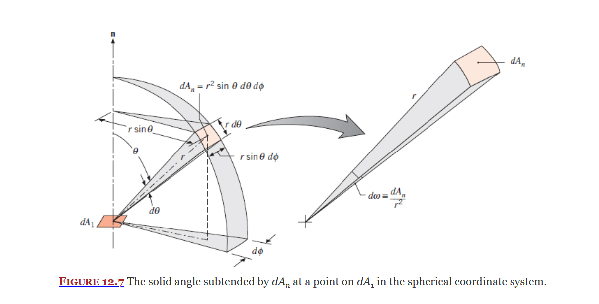
Where refers to integration over the hemisphere.

The unit of the solid angle is steradian (sr), equal to radians for plane angles?

14A - 2nd Class

solid-angle

Spectral Intensity

Defined in Section 12.3.2 by Equation 12.10:

Where is wavelength, and are angles as defined in radiation intensity.

14A - 2nd Class, 14C - 2nd Class

spectral-intensity

Radiation

Covered in Chapter 12 and 13, radiation is heat transfer due to changes in election configuration, it takes the form of electromagnetic waves.

Radiation exists on electromagnetic radiation spectrum (Figure 12.3 below), a subset of this spectrum is thermal radiation which is what this course focuses on. Thermal radiation is an electromagnetic wave.

From 13E - 2nd Class:

Thermal radiation is measured via four different radiation heat fluxes defined in table 12.1:

See ME3304 S24 Lecture Note (7) Radiation for more info.

Tip

When working with radiation, Dr. Paul recommends to always convert to Kelvin.

radiation-balance
radiation-intensity
view-factor

radiation

Radiation Balance

Section 12.6

Radiation Balance is defined in Equation 12.46:

Where is irradiation and is wavelength.

radiation-balance

Opaque Medium

An opaque medium just means there is no radiation that makes it all the way though.

- Dr. Paul

Where is transmissivity.

opaque-medium

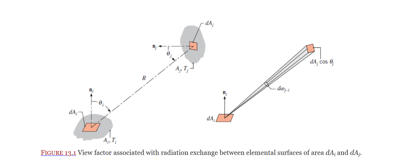
View Factor

Covered in Section 13.1, the view factor is defined by the book as the fraction of radiation leaving surface i that is intercepted by surface j.

View factors for 2D geometries can be found on table-13.1.
View factors for 3D geometries can be found on table-13.2.

Rules / Relations

Reciprocity Relation (Eq. 13.3):

Summation Rule (Eq. 13.4) for surfaces in an enclosure:

Where is the number of surfaces.

See ME3304 S24 Lecture Note (7) Radiation and 15A - 2nd Class for more information.

view-factor

Fick's Law

Covered in Section 14.1.3, Fick's Law is like Fourier's law but applied to mass transfer.

Equation 14.12:

Where is diffusive mass flux of species A, is density, is mass diffusion of species A into B, is the mass of species A.

Equation 14.13:

Where is the diffusive molar flux, is molecular concentration, is the diffusion of species A into B, and is the mole fraction of species A.

See ME3304 S24 Lecture Note (8) Mass Transfer for more information.

ficks-law

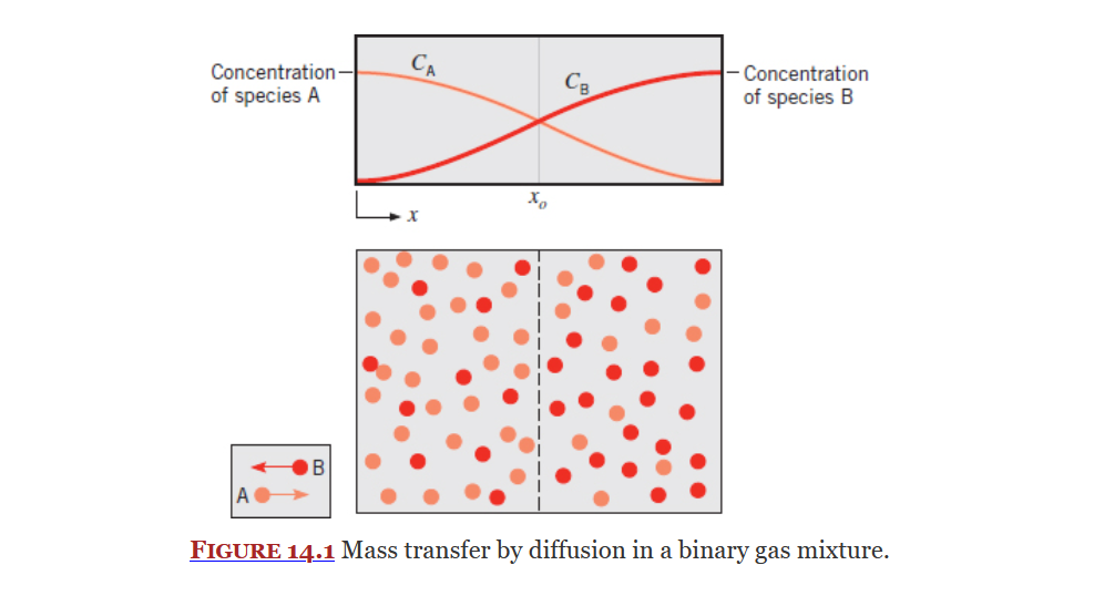
Mass Diffusion

Covered in Chapter 14, mass diffusion is the diffusion (or movement) of mass from a high concentration to an area low concentration.

Where is species A (a species is simply a grouping, it could be an element, chemical, or other) and is species B. The above variable is the diffusion of species A into species B.

Equation 14.14 (Slide 8 of ME3304 S24 Lecture Note (8) Mass Transfer):

Where is temperature in Kelvin, is mean speed of sound, is electron mean free path, is pressure, and is temperature.

See ME3304 S24 Lecture Note (8) Mass Transfer for more information.

mass-diffusion

The Three Heat Transfer Methods

Conceptual Ideas